


 nueva página del texto (beta)
 Inglés (pdf)
 Artículo en XML
 Referencias del artículo
 Enviar artículo por email
 Citado por SciELO
  Similares en
SciELO
Similares en
SciELO 
 Permalink
1 Introduction
In recent years, the problem of HAR has received a lot of attention from researchers. This is because today it is common to find problems related to video surveillance, behavior analysis or Human Computer Interaction (HCI) [1].
The first attempts to solve this problem using hand crafted features such as Histogram of Oriented Gradients (HOG), Histogram of Optical Flow (HOF) or Motion Boundary Histogram (MBH) [2-6]. However, the main issue of using these types of approaches is that it is difficult to transfer the handcrafted features of a training dataset to another [7]. This issue was solved by the introduction of convolutional neural networks (CNN), which are able to automatically detect features in raw images, to find the connection between them and use the learned features of a training dataset to train a different dataset [8-13].
With the breakthrough that CNN caused in 2012 in the machine vision community given their tremendous reduction of error rates of up to 20% to closest participants, it was clear that CNN would be the approach to exploit in image/video classification problems. In fact, two of the three most popular approaches (two-stream and 3DCNN) use CNN as a pillar while the third one uses recurrent neural networks [13].
One of the main questions when building a HAR model is which CNN to use, since every year there are new state-of-the-art CNN architectures on the ImageNet dataset. One may think that using the CNN with the top performance on the ImageNet dataset can achieve the best results. The main issue of thinking this way is that is not taking into consideration that the CNN was trained to classify images with any object class of the 1000 classes that the ImageNet dataset has and not frames of human actions, which they are the main components of the videos in a HAR dataset. With this in mind, the main objective of this work is to prove that a CNN with the best performance on the ImageNet dataset does not always achieve the best results on a video dataset, thus it is important to test different CNNs under the same conditions when building a HAR model.
Regarding the originality of this study, we argue that even when new CNN models appear practically every year, very little is known regarding how these models compare to each other, or even against the previous competitive proposals, over the HAR problem, since no systematic and exhaustive experimental comparison, to the best of our knowledge, had been done until now.
This work makes an analysis of comparison about training time and accuracy of 8 different CNN architectures using different sets of RGB images that were built from the videos of the HMDB51 dataset. The CNN models were trained as image classifiers and it was used the average of the predictions of each image frame to generate the classification label of the activity in video. Lastly, different ensembles were considered using the best accuracy performance on the CNN architectures to prove if there is an increment in the accuracy using ensemble predictions.
The main contribution of this study is twofold. First, we empirically show that for a CNN having top performance on the Imagenet dataset does not imply top performance on the HAR task, as it usually is assumed by the community. This opens up important questions regarding what would be the best experimental setting for these neural models to achieve better results on such task.
Additionally, we tackle a long standing question for the HAR problem, which is to make the first exhaustive evaluation that considers up to 8 different state-of-the-art CNN-based approaches under very similar experimental settings that will allow to have the first impressions of who is who regarding performance and efficacy for Human Action Recognition endeavors. As a whole, with these results, the community will have enough evidence regarding what baseline model to use from now on, this being the Xception network, to compare their new contributions against.
2 Related Work
This section includes a description of previous works related to the HAR problem using the HMDB51 dataset. We made a revision based on the three main approaches for handling the HAR problem. It is important to note, that this work is not going to consider all the approaches revised here and the papers cited are only to tell the viewer what has been done in relation to HAR using the HDMB51 dataset and which CNNs are the most used among researchers on this field.
Two-stream approach was proposed by Simonyan et al. in 2014 [15] by the idea that they can have a CNN trained with raw RGB frames and another CNN trained with optical flow, which represents the moving vectors between two consecutive frames. They later combined the predictions of the two-streams using a weighted averaged of the predictions. Each stream had a CNN called ClarifaiNet and their best accuracy was 59.4%.
Wang et al. [16] decided to divide a video into 3 segments so that each segment have their own two-stream network and then combine the predictions of all segments of a certain stream and after that combine the stream predictions. All segments of all streams used the Inception-V2 CNN and they obtained an accuracy of 69.4%.
Zhu et al. [17] designed an architecture that was able to combine the feature vector of different frames into a video representation by using max pooling and a pyramidal layer. They also used Kinetics as the pre-trained dataset for the CNN, which result in better accuracy than using the ImageNet dataset. They also used Inception-V2 and their best result was an 82.1% in accuracy.
Cong et al. [18] developed an adaptive batch size K-step model averaging algorithm (KAVG). They customized the Adam optimizer and proposed to use a network to determine the best optical flow images from RGB frames. They attached that model to the two-stream network to form a three-stream network, which increases their accuracy even more. For the three streams, they used the ResNet152 network obtaining an 81.24% in accuracy.
He et al. [19] added an additional stream to the two-stream approach, which it was able to fuse the features of a frame with the features of its two neighbor frames. This was done several times with the purpose of improve the frames features and that proved to be beneficial for the model. The CNN they chose was Inception-V2 obtaining a 73.1% in accuracy.
Wan et al. [1] proposed to combine the 3DCNN approach with the two-stream approach by using 3D convolutions on the spatial-stream and the VGG16 CNN on the temporal-stream. They also used a SVM after the combination of the two-stream features for the final prediction and obtained a 70.2% in accuracy.
Sun et al. [20] preferred to use a 3DCNN to model the relationship between the features of multiple frames, but instead of using a 3D convolution, they decided to divide the convolution in a set of 2D convolutions followed by a 1D convolution to model the temporal relationship between frames. They created their own 3D CNN and their best result was 59.1% in accuracy.
Carreira et al. [21] combined the two-stream approach with the 3DCNN approach by using a 3D CNN in both streams. They also proposed to use the Kinetics dataset for pre-training instead of the ImageNet dataset. The 3D CNN is based on Inception-V1 and it was called I3D CNN. The best result obtained was 80.9% in accuracy.
Wang et al. [22] used the I3D CNN proposed by Carreira et al. to build an architecture capable of learning the Fisher vector and bag of words representation of a combination of features extracted from RGB and optical flow frames. Their best result showed an 82.1% in accuracy.
Piergiovanni et al. [23] designed an evolving algorithm, which it was able to create convolutional models with different number and type of layers for the best detection of spatial and temporal features in videos. The model is based on Inception-V1 and the best result was 82.1% in accuracy.
Yang et al. [7] also attacked the computational cost of the 3D convolutions just like Sun et al. [20] but they used unidirectional asymmetric 3D convolutions. They also made their own CNN architecture achieving a 65.4% in accuracy.
Stroud et al. [24] proposed a model called D3D, which it was trained with RGB frames and with extracted knowledge of a temporal network trained with optical flow images. The CNN that they used was a 3D CNN called S3D-G and it is based on the I3D CNN. Their best result showed an 80.5% in accuracy.
Sharma et al. [25] chose to make a visual attention model using the Inception-V1 CNN as a feature extractor, an attention mechanism that was in charge of selecting which parts of the feature tensor were the most important ones and an RNN to model the relationship between the most important features of each frame. Their best result was a 41.3% in accuracy.
Ye et al. [26] proposed to combine the features of the last convolutional layer of each of the two ResNet101 CNN in a two-stream network and feed the combined feature vector to a convolutional LSTM to make the final prediction. They obtained a 69.3% in accuracy.
Outside HMDB51 dataset there is also numerous works on HAR in videos using different datasets. For example, He et al. [27] proposed to create a high accuracy architecture based on the integration of information from audio, RGB frames and two different types of optical flow images. They used ResNeXt101 and InceptionResNetV2 CNNs on their experiments. The Kinetics 400 database was used for pre-training and the final training and evaluation were on the Kinetics 600. The best accuracy was 85% using an ensemble of individual models.
Donahue et al. [28] decomposed the video into frames; each frame entered to a CNN to extract its characteristics and then passed to a LSTM. The prediction of each LSTM was averaged to have the final video tag. The base architecture in their experiments was a combination of the CaffeNet architecture and another network proposed by other authors. They got 82.37% accuracy in the UCF101 dataset.
Yue-Hei Ng et al. [29] experimented with various numbers of frames, various CNN architectures such as feature extractors (AlexNet and Inception-V1), various feature grouping architectures, and a recurring network in order to model a higher level of temporal features between frames in the video. They used the UCF101 database, obtaining an 88.6% accuracy.
Limin et al. [30] used UCF101 dataset. A valuable observation about their work is that they used 3 different CNNs (ClarifaiNet, GoogleNet and VGG16) on their experiments and the results showed that VGG16 outperforms GoogleNet, which is interesting because the later performs better on ImageNet dataset. Although they did not train their CNNs under the same circumstances, due to the random corner-center cropping and random resizing techniques that they applied to the frames, this last work is an example of why we do not have to assume that a single CNN will be the best on every single dataset in existence.
3 Theoretical Background
3.1 Artificial Neural Networks (ANN)
The ANN is a machine learning (ML) algorithm based on the operation of neurons in the human brain. ANN uses mathematic equations to learn patterns of the training data and they are made up by the union of multiple units called perceptrons.
Frank Rosenblatt made the perceptron and he defined it as an artificial neuron that receives multiple inputs and produces one binary output that is feed to the next neuron. A perceptron also receives the name of neuron [31].
Equation (1) shows the process of calculating the output of a neuron, where
The following are some of the activation functions that can be used on a neuron [31]:
− Sigmoid function: It is an S-shaped function and it converts the input values into probabilities between 0 and 1.
− Softmax function: It is commonly used in the output layer of neural networks in classification algorithms. Computes the probability of the output being one of the target classes compared to the other classes.
− Tanh: This function represents the relationship between the hyperbolic sine and the hyperbolic cosine. It is S-shaped and converts input values to probabilities between -1 and 1.
− ReLU: It is conventionally used in the hidden layers of neural networks. It works in such a way that, if the input is greater than 0, the output is the same input value; if it is less than 0, the output is equal to 0.
The process of all the calculations that are made from left to right through all the neurons in an ANN is called “forward propagation”. The output of this process is used to generate the error of the network in comparison to the target. The error is used to adjust the network parameters (weight and bias), and that adjustment process is called back propagation [31].
3.2 Convolutional Neural Networks (CNN)
In an ANN each neuron in the input layer is connected to each neuron on the subsequent layer, this is known as a dense layer. However, in a CNN, a dense layer is not used until the last layers of the networks. In this way, a CNN can be defined as a neuronal network that exchanges a dense layer for a convolutional layer in at least one layer of the network [32].
A convolution can be defined as the sum of the element-wise multiplication between the values of the filters that overlap the values of the input tensor. A convolution takes into consideration the spatial relationship between pixels and its main goal is to extract useful features from the input tensor [33].
Nonlinear functions such as ReLU are applied to the output of the convolutions and then the new output is passed to the next layer and the process continues. A CNN also includes a pooling layer, which it helps to reduce the width and height of the input tensor [32].
Finally, the feature tensor is flattened to produce a 1-dimensional vector, which it is feed to one or more dense layers to make the predictions [32].
In practice, CNNs provide two key benefits: local invariance and compositionality. The concept of local invariance allows to classify an image that contains a particular object, regardless of where in the image the object appears. This local invariance is obtained by using "pooling layers" that identify regions in the input volume with a high response to a particular filter. The second benefit is compositionality. Each filter composes a local patch of lower-level features into a higher-level representation, similar to how you can compose a set of mathematical functions that are based on the output of previous functions. This composition allows the network to learn richer features and deeper into the network.
For example, the network can build edges from pixels, shapes from edges, and then complex objects from shapes, all in an automated manner that occurs naturally during the training process [32].
Figure 1 shows an example of an architecture CNN, where F1, F2 are the number of feature maps on each layer and C1 and C2 are the number of neurons in each dense layer.

3.2.1 CNN Architectures
In this section, we are going to review some important characteristics of the CNN architectures that will be considered later in the analysis. Since most of the literature revised use Inception-V1 or Inception-V2, we decided to consider the most similar one that belongs to the Keras library for python, which was Inception-V3.
Inception-V3 [34] is a 48-layer CNN and its main difference from the Inception-V2 CNN is that
DenseNet201 [36] was selected because it is the best of all DenseNet CNNs and because it introduced the concept of dense connections between features maps. This proved to be beneficial because it solves the vanishing gradient problem as ResNet did and at the same time, it maintains the low-level features through all the convolutional layers within a dense block. it uses RMSProp Optimizer, 7x7 factorized convolutions, batch normalization in the auxiliary classifiers and label smoothing, which is a type of regularizing component added to the loss formula that prevents the network from becoming too confident about a class avoiding the overfitting.
ResNet architectures family are also common in the revised works, we decided to consider ResNet152 [35] because we want to compare only the most accurate CNN within a group of related CNN. ResNet152 is a 152-layer CNN and its CNN family was the first that attacked the problem of vanishing gradient by using residual connections and residual blocks. A residual block is a stack of layers set in such a way that the output of a layer is taken and added to another layer deeper in the block using a residual connection. Finally, a non-linearity is applied to the result of the sum.
For the comparative analysis, the remaining CNN architectures were chosen from the Keras library, according to the next criteria. Since we work with the Keras library to get the previous CNNs architectures, we decided to also compare some of the other CNNs that the Keras library offers to work with.
The Xception [37] CNN stands for an extreme version of Inception and has 36 convolutional layers and was chosen because it proposed the use of modified Depthwise Separable Convolutions (DSC) with no intermediate non-linearity. These types of convolutions were stacked in the Xception model like Inception modules and the Xception accuracy on ImageNet probed to be better than InceptionV3, so we wanted to know if this feature was maintained with the HMDB51 dataset.
The EfficientNetB0 [38] and EfficientNetB3 [38] CNNs are part of a large family of CNNs known as EfficientNet. There are CNN architectures going from EfficientNetB0 all the way to EfficientNetB7.
At first, we used 3 CNNs of this family, EfficientNetB0, EfficientNetB3 and EfficientNetB7, but we decide to skip the use of EfficientNetB7 in the experiments because the difference in accuracy between EfficientNetB3 and EfficientNetB7 was not significant and the number of parameters increased.
The main contribution of this type of CNNs is the introduction of compound scaling which uniformly scales network width, depth, and resolution with a set of fixed scaling coefficients.
For instance, if the aim is to use 2N times more computational resources, then the network depth can increase by αN, width by βN, and image size by γN, where α, β, and γ are constant parameters computed by a small grid search on the original small model.
EfficientNet uses a compound coefficient ø to uniformly scale the width, depth, and resolution of the network in a novel manner. The use of the compound scaling method is justified since, when the input image is bigger, the network needs additional layers and channels to increase the receptive field and to capture more fine-grained patterns on the bigger image, respectively.
Finally, we decided to select MobileNetV2 and NASNetMobile from Keras library to compare the accuracy of mobile CNNs in respect to the other ones. MobileNetV2 [39] is a 53-layer CNN and is the successor of MobileNetV1 which introduced the concept of DSC which dramatically decreased the number of parameters in the network. MobileNetV2 like its predecessor uses DSC, but non-linearities in narrow layers are removed this time, which was beneficial for the model classification performance. It also introduced inverted residual blocks (as opposed to ResNet) to improve parameter efficiency.
NASNetMobile [40] CNN is part of the NASNet CNN family and it was built using reinforcement learning using an RNN that selected the best combinations between a predefined set of states and actions, these combinations are called blocks. The main idea behind this approach was to make use of transfer learning by searching for an architectural building block that work on a small dataset (CIFAR10) and then transfer the block to a larger dataset (ImageNet). It is also introduce a new regularization technique called ScheduledDropPath which improved the generalization of the NASNet models.
4. Methodology
4.1 HMDB51 Dataset
HMDB51 is a 6766-video dataset with 51 human action classes and for each class there are at least 100 videos. The dataset has 3 sets of videos for training and testing.
The spatial resolution of the videos is 320x240 pixels. All videos were extracted from YouTube or digitalized movies. The dataset can be downloaded using this linkfn.
4.2 Set of Frames
By the intuition that the random selection of frames in the training stage of a CNN affects the accuracy of the architecture, we decided to create 4 different sets of frames for the use in all CNNs. All frame sets described here used the videos from the set 1 of the HDMB51 dataset.
4.2.1. First Set of Frames
This set of frames was built taking 10 evenly spaced frames from each training and testing video. The frames extracted from the training videos were saved in a different folder that the ones extracted from the test videos.
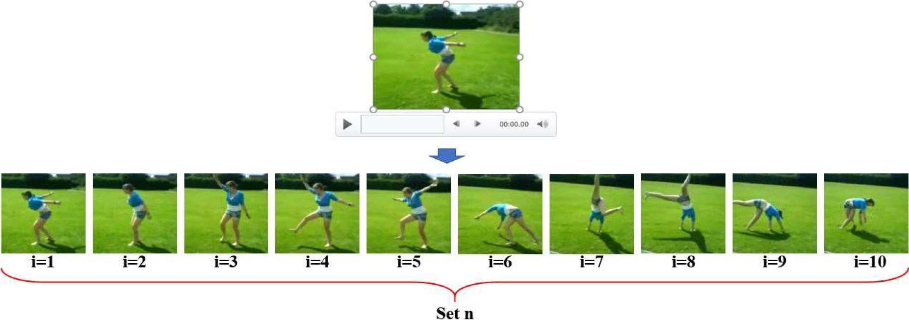
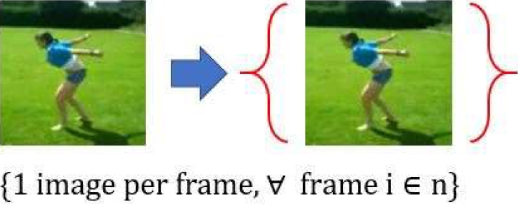
To extract the frames, first the program gets the total number of frames in the video and this value is divided by 10 to calculate the position between each frame that will be extracted. Finally, the program saves the index of each frame and if the quotient between the frame index and the position between frames is zero, then the frame is extracted. Since the index for the first frame is 0, the first frame of the video is always extracted (see Fig. 2). For this set of frames, we did not include any sort of image augmentation, so there is only one image per frame (see Fig. 3).
4.2.2 Second Set of Frames
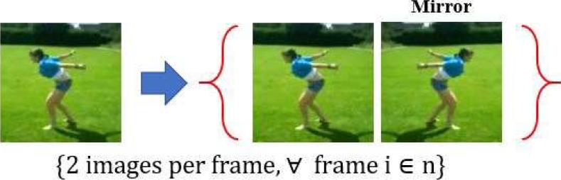
With the aim of evaluating the effect of data augmentation, we decided to use 3 different techniques. The first one used in this set of frames considers the horizontal mirror of each frame, so that instead of having 10 frames per video, this set of frames will have 20 frames (10 original and 10 horizontal mirror). The saving and extraction of the frames is as described in the first set of frames (see Fig. 4).
4.2.3 Third Set of Frames
The second data augmentation technique consists of resizing each frame to 256x256 pixels, and from the resized frame cut a 224x224 region from the center to each one of the four corners. This process generated 5 sub-frames from each frame, so at the end each video will have 50 frames (40 frames in total from all the corners and 10 central frames). The saving and extraction of the frames is as described in the first set of frames (see Fig. 5).

4.2.4 Fourth Set of Frames
The third data augmentation technique consists of resizing each frame to 256x256 pixels, and from the resized frame cut a 224x224 region from the center to each one of the four corners. After that, we took the horizontal mirror from each one of the 5 generated images. This process generated 10 subframes from each frame, so at the end each video will have 100 frames (80 frames in total from all the corners plus their mirrors and 20 frames from the center of each one and its mirror). The saving and extraction of the frames is as described in the first set of frames (see Fig. 6).

4.3 Ensembles
For the experiments with ensembles, we considered the best CNN architectures. Each ensemble was built by 3 or 5 CNN architectures and we used 5 different methods based on averaging and voting to obtain the final classification tag for each video. All CNN architectures were trained with the same set of frames. Each one of the 5 methods is described below.
4.3.1 Using Simple Voting with n Frames of Each Test Video
This method consists of extracting 10 frames evenly spaced and applying the corresponding image augmentation technique according to the set of frames used for training. Each frame of the set passes through all the CNNs in the ensemble and they generate a tag and a number which are added to a label dictionary. The key stored within the dictionary corresponds to the tag predicted by at least one of the CNNs and the number of classifiers that predicted that tag. To obtain the final tag, the voting method was used where the tag that had the most votes by CNNs within thedictionary is used to establish the final tag for the video (see Fig. 7).

4.3.2 Using Simple Voting with All Frames of Each Test Video
This method works exactly as the previous method; the only difference is that instead of using only 10 frames we used all the frames in the test video.
This was done with the purpose of seeing the change in accuracy when considering all the frames of the video.
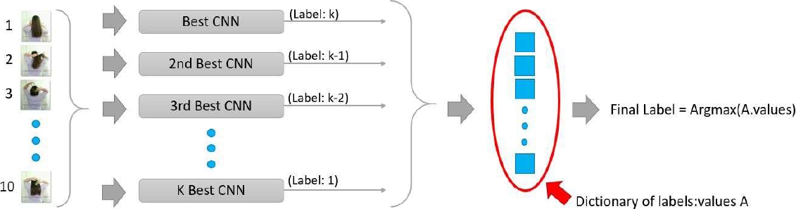
4.3.3 Using Weight Voting with n Frames of Each Test Video
This method consists of extracting 10 frames evenly spaced and applying the corresponding image augmentation technique according to the set of frames used for training.
Each frame of the set passes through all the CNNs in the ensemble and they generate a tag and a value which are added to a label dictionary.
The key stored within the dictionary corresponds to the tag predicted by at least one of the CNNs and the value is the weight referred to the CNN. The weight of each CNN was determined according to its individual performance in experiments before ensembles.
The best CNN has a weight of k, the second best has a weight of k-1, and this continues until we reached the weight of 1.
This was done for proving if exist any significant difference between simple and weighted voting method when taking in consideration the individual performance of each CNN.
To obtain the final tag for the video, we looking for the tag with the greater score within the dictionary (see Fig. 8).
4.3.4 Using Prediction Averaging with n Frames of Each Test Video
This method consists of extracting 10 frames evenly spaced and applying the corresponding image augmentation technique according to the set of frames used for training. Each frame of the set passes through all the CNNs in the ensemble.
Each CNN generates n predictions, which are stored in a matrix of predictions. The final tag for the video is obtained by averaging all the predictions of all CNN in the prediction matrix, which gives us a vector with C classes.
Finally, we took the index that has the greater value in the vector to generate the corresponding tag (see Fig. 9).

4.3.5 Using Prediction Averaging with All Frames of Each Test Video
This method works exactly as the method of section 4.3.4; the only difference is that instead of using only 10 frames we used all the frames in the test video.
This was done with the purpose of seeing the change in accuracy when considering all the frames of the video.
4.4 Our Proposal
The main purpose of this work is to make an analysis of comparison about training time and accuracy of 8 different CNN architectures using the HMDB51 dataset.
By no means has it intended to achieve a better accuracy than cited works. The training of each CNN architecture was done by using only RGB frames from the set of videos of the HMDB51 dataset.
By this statement, our proposal is to treat each CNN as an image classifier leaving aside the three popular approaches for the HAR problem. To make a prediction of human action in the video, we averaged the predictions of all the frames in a given test video.
4.5 Environment Setup
We used python as the programming language. Regarding training variables, we used the default input tensor dimension for all CNNs and the batch size that we used was set to 16.
For the learning rate, we used the default value that each optimizer has in Keras; refer to https://keras.io/api/optimizers/ for more details. Since the default image size is 299x299 for InceptionV3 and Xception CNNs, we resized the frames to have that size and take advantage of the pre-trained weights of those CNNs. All other CNNs work with 224x224 size.
We ran the experiments in 3 different computers each one with a different GPU. The GPUs that we used were as follows: NVIDIA 1060, NVIDIA 1080 and NVIDIA TITAN RTX. The main libraries used were: Keras implementation in TensorFlow, efficientnet, NumPy, OS, OpenCV, Shutil and Pickle.
We used Tensorflow as a backend to run the CNN experiments. We loaded most of the CNN architectures using the module of Keras library except for the EfficientNet CNNs in which case we used the efficientnet library. The metric that was used to measure the performance of the CNNs was accuracy in all experiments. In some experiments, we also measured the training time in different GPUs for all the CNNs.
5 Experiments and Results
The first experiment consists of selecting the best optimizer to use in all CNNs. For this, we considered 5 different optimizers: “Adagrad”, “Adam”, “Nadam”, “RMSprop and “SGD” with their default values in Keras library. We used a K-Fold of 3 to validate our results. For this, we divided the training videos of set 1 in 2 folders, 70% of the videos were used for training and 30% for validation.
Since each one of the 51 folders (classes) in the HMDB51 dataset has 70 videos, each class was divided in 49 videos for training and 21 videos for validation. To extract the frames of each video in both the training and validation folders, we used the process described in 4.2.1 section.
Each fold was run 5 times to mitigate the bias produced by random weight initialization on the CNNs that was used. Due to the excessive time that it would take to train 15 times each CNN for each optimizer, we decided to use a less deep CNN only for the first three experiments. The CNN architecture is the following [41]:
– An input layer where the dimension for the input tensor is 224x224x3.
– A convolutional layer with 32 filters of 3x3 followed by a “ReLU” activation function and a 2x2 maxpooling.
– A second convolutional layer with 32 filters of 3x3 followed by a “ReLU” activation function and a 2x2 maxpooling.
– A third convolutional layer with 64 filters of 3x3 followed by a “ReLU” activation function and a 2x2 maxpooling.
– A flatten layer followed by a dense layer of 64 neurons with “ReLU” activation function, a Dropout layer with a value of 0.5 and a final dense layer with 51 neurons with a “softmax” activation function.
The training was done for 50 epochs and the model with the best validation accuracy (Val_Acc) as well as the model with best validation loss (Val_Loss) were saved. For the validation phase, the final label of the video was obtained by averaging the predictions of the n frames generated of each validation video. The results showed the average accuracy of the 5 best Val_Acc and the 5 best Val_Loss models in the validation set on each fold (see Table 1).
Table 1 Average accuracy of each optimizer in each fold using the best models and the first set of frames
| Optimizer | Model | Fold 1 | Fold 2 | Fold 3 | Average |
| Adagrad | Val_Loss | 43.49% | 39.12% | 40.22% | 40.95% |
| Val_Acc | 44.03% | 39.70% | 40.69% | 41.48% | |
| Adam | Val_Loss | 39.48% | 37.42% | 37.89% | 38.26% |
| Val_Acc | 44.67% | 43.29% | 42.80% | 43.59% | |
| Nadam | Val_Loss | 42.58% | 40.60% | 36.00% | 39.73% |
| Val_Acc | 47.19% | 45.90% | 43.21% | 45.43% | |
| RMSprop | Val_Loss | 43.12% | 38.45% | 40.95% | 40.84% |
| Val_Acc | 42.73% | 40.54% | 42.84% | 42.04% | |
| SGD | Val_Loss | 43.90% | 40.02% | 39.74% | 41.22% |
| Val_Acc | 47.26% | 45.23% | 44.41% | 45.63% |
The second experiment was realized almost exactly as the first one, but instead of extracting the frames using the previous process, we use the process of section 4.2.2. This was done with the main purpose of observing if any optimizer performs better than others when considering a larger number of frames (see Table 2).
Table 2 Average accuracy of each optimizer in each fold using the best models and the second set of frames
| Optimizer | Model | Fold 1 | Fold 2 | Fold 3 | Average |
| Adagrad | Val_Loss | 45.83% | 42.65% | 40.97% | 43.15% |
| Val_Acc | 46.05% | 42.75% | 41.29% | 43.36% | |
| Adam | Val_Loss | 44.76% | 43.01% | 43.59% | 43.78% |
| Val_Acc | 50.59% | 49.67% | 48.24% | 49.50% | |
| Nadam | Val_Loss | 48.57% | 43.53% | 43.83% | 45.31% |
| Val_Acc | 53.80% | 50.03% | 49.41% | 51.08% | |
| RMSprop | Val_Loss | 41.89% | 39.25% | 40.11% | 40.42% |
| Val_Acc | 43.87% | 39.23% | 42.04% | 41.71% | |
| SGD | Val_Loss | 49.04% | 45.62% | 44.26% | 46.31% |
| Val_Acc | 53.71% | 51.39% | 49.71% | 51.60% |
Based on the previous results, we decided to use SGD optimizer for the training of all the CNNs in the next experiments. For the third experiment, we measure the training time of all the CNNs architectures with the frames of the set 1. We trained each of the CNNs 3 times for 50 epochs. The CNNs were pre-trained with the ImageNet dataset. We reported the average running time of each CNN in seconds when using a GPU 1080 and a GPU TITAN RTX (see Table 3).
Table 3 Running time in seconds of each CNN architecture on a Titan RTX and 1080 GPU.
| CNN | TITAN RTX | 1080 |
| EfficientNetB0 | 9133 s | 18717 s |
| EfficientNetB3 | 17464 s | 35321 s |
| Xception | 28549 s | 61730 s |
| InceptionV3 | 12033 s | 26869 s |
| ResNet152 | 20878 s | 49355 s |
| DenseNet201 | 15239 s | 33675 s |
| MobileNetV2 | 7034 s | 12913 s |
| NASNetMobile | 14025 s | 25519 s |
From Table 3 we can observe that the fastest CNN is the MobileNetV2 architecture, which is understandable because it contains the lowest number of parameters. An interesting fact is that the Xception CNN is from 2 to 3 times slower than the Inception CNN and they share almost the same number of parameters. We decided to conduct another experiment to understand why that happened.
For the fourth experiment, we used the GPU 1060 and computed the average of the training time of 5 epochs on both CNNs. We also measured the average prediction time of 5 epochs, which was calculated by measuring how much time the CNN needed to make a prediction of all the training frames. Finally, with both times we calculated the time that the CNNs used to update their weights by extracting the average prediction time to the average training time (see Table 4).
Table 4 Prediction, updating and training time of Xception CNN and InceptionV3 CNN
| CNN | Prediction | Updating | Training |
| Xception | 389.17 s | 1538.89 s | 1928.06 s |
| Inception | 226.90 s | 612.48 s | 839.38 s |
With the previous results, we observed that even if both CNNs share almost the same number of parameters, the inner structure of the Xception CNN made the network slower than the InceptionV3, especially when we compared the updating time of both networks.
In the fifth experiment, we trained all the CNNs with each one of the four different sets of frames. For the third and fourth set of frames, we decided to train only four CNNs due to the excessive training time since this process is carried on using one GPU. We trained each one of the CNNs three times for 50 epochs. The CNNs were pre-trained with the ImageNet dataset. For each set of frames, we used the corresponding testing frames for validation and we saved the model with the best validation accuracy for testing. For the testing phase, the final label of each video is obtained by averaging the predictions of the n frames generated from each test video according to the set of frames used during training. We reported the average accuracy of the 3 runs of each CNN on the testing videos for each set of frames used during training (see Table 5).
Table 5 Average accuracy of each CNN on each set of frames
| CNN Architecture | 1st set | 2nd set | 3rd set | 4th set |
| EfficientNetB0 | 47.39% | 49.67% | 51.35% | 48.17% |
| EfficientNetB3 | 47.84% | 50.70% | N/A | N/A |
| Xception | 51.33% | 53.99% | 52.68% | 50.26% |
| InceptionV3 | 48.21% | 48.56% | 48.39% | 46.95% |
| ResNet152 | 44.81% | 45.80% | N/A | N/A |
| DenseNet201 | 45.95% | 45.99% | N/A | N/A |
| MobileNetV2 | 42.53% | 43.75% | N/A | N/A |
| NASNetMobile | 43.86% | 44.47% | 45.40% | 44.18% |
According to the results of the previous experiment, we noticed that all the CNNs were benefited from using the second set of frames, but on the third one, only two of the four CNNs improved their accuracy. What is even more interesting and that none of the four CNNs that were trained on the fourth set of frames improved their performance, instead of that, the performance was worse than when using the second and third set of frames.
This result can be explained by the fact that when building the first and second set of frames, we worked with the whole image, but when building the third and fourth set of frames, we took five different subsections of the whole image and some of them did not contain the person doing the action. With this in mind, we can argue that both the third and fourth set of frames have many frames with noise, and that is why the accuracy performance on these two sets was affected negatively. Based on that information, we decided to not train any of other remaining CNNs on the 3rd and 4th set of frames. Since the 2nd set of frames prove to be the set with better results on the CNNs, we used that set for the training of the CNNs for the next experiments.
The sixth experiment was done with the purpose of proving how well the CNNs perform on the set 2 and set 3 of videos of the HMDB51 dataset. Aiming at this, we used the procedure described in section 4.2.2 to generate new sets of frames from the sets 2 and 3 of videos of the HMDB51 dataset. We trained each one of the CNNs 3 times for 50 epochs. The CNNs were pre-trained with the ImageNet dataset. For each set of frames, we used the corresponding testing frames for validation and saved the model with the best validation accuracy for testing. For the testing phase, the final label of each video was obtained by averaging the predictions of the 20 frames generated from each test video according to the set of frames that was used during training. We reported the average accuracy of the 3 runs of each CNN in the testing videos for each set of frames used during training and included the results obtained in the set 1 of videos using the second set of frames from the previous table (see Table 6).Something that caught our attention on the result of the fifth and sixth experiment was the fact that the Xception network proved to be better than the EfficienNetB3 network, which is on a higher rank on the ImageNet dataset.
Table 6 Average accuracy of each CNN on each of the three set of videos of HMDB51 dataset.
| CNN Architecture | Set 1 HMDB51 | Set 2 HMDB51 | Set 3 HMDB51 | Average |
| EfficientNetB0 | 49.67% | 45.62% | 45.66% | 46.98% |
| EfficientNetB3 | 50.70% | 46.97% | 45.88% | 47.85% |
| Xception | 53.99% | 50.00% | 51.76% | 51.92% |
| InceptionV3 | 48.56% | 46.25% | 47.25% | 47.35% |
| ResNet152 | 45.80% | 39.96% | 40.46% | 42.07% |
| DenseNet201 | 45.99% | 42.42% | 43.75% | 44.05% |
| MobileNetV2 | 43.75% | 41.33% | 41.22% | 42.10% |
| NASNetMobile | 44.47% | 40.04% | 40.76% | 41.76% |
For knowing if these results were caused by the greater entry resolution of the Xception network, we decided that the aim of the seventh experiment would be to compare these two networks with the same input resolution.
We fixed the input resolution of each of the two CNNs to be 224x224 and trained both CNN for 50 epochs on the second set of frames of the set 1 of videos of HMDB51. The CNNs were pre-trained with the ImageNet dataset. We used the testing frames of the second set of frames for validation and saved the model with the best validation accuracy for testing. For the testing phase, the final label of each video was obtained by averaging the predictions of the 20 frames generated from each test video. We reported the average accuracy of the 3 runs of each CNN in the testing videos (see Table 7).
Table 7 Accuracy of EfficientNetB3 and Xception using 224x224 images.
| CNN Architecture | Accuracy |
| EfficientNetB3 | 50.70% |
| Xception | 52.46% |
Based on the previous results, we can see that even when both CNNs have the same input resolution, the Xception CNN managed to outclass the EfficientNetB3 CNN by a significant margin.
We can also see that the Xception network works better with a 299x299 input image resolution and that is due that input images of 299x299 resolution were used to generate the pre-training weights of the Xception CNN on the ImageNet dataset.
The eighth experiment was envisioned to take advantage of those CNN models that showed the best performance on previous evaluations. For this, we thought of building several ensembles made of such CNN's to evaluate if they could, as a team, outperform the best individual model for HAR, that is, Xception. If that is the case, then, this ensemble can also be considered as a baseline for future evaluation. Since we trained 3 times each CNN, we selected the CNN model which test accuracy was the closest to the average that was reported on each set of videos to be part of the ensembles.
We decided to separate the ensembles that considered only n frames (n = 20) of each test video and the ones that considered all video frames of each test video. The ensembles were formed in the following way:
– Ensemble 1: Ensemble of the 3 best CNNs using simple voting and n frames.
– Ensemble 2: Ensemble of the 5 best CNNs using simple voting and n frames.
– Ensemble 3: Ensemble of the 3 best CNNs using weighted voting and n frames.
– Ensemble 4: Ensemble of the 5 best CNNs using weighted voting and n frames.
– Ensemble 5: Ensemble of the 3 best CNNs using prediction averaging and n frames.
– Ensemble 6: Ensemble of the 5 best CNNs using prediction averaging and n frames.
– Ensemble 7: Ensemble of the 3 best CNNs using simple voting and all frames.
– Ensemble 8: Ensemble of the 5 best CNNs using simple voting and all frames.
– Ensemble 9: Ensemble of the 3 best CNNs using prediction averaging and all frames.
– Ensemble 10: Ensemble of the 5 best CNNs using prediction averaging and all frames.
We reported the average accuracy of each ensemble in each set of videos of the HMDB51 dataset (see Table 8).
Table 8 Accuracy of the different type of ensembles on each set of videos of HMDB51 dataset
| Ensemble | Set 1 HMDB51 | Set 2 HMDB51 | Set 3 HMDB51 | Average |
| Ensemble 1 | 52.88% | 48.30% | 50.00% | 50.39% |
| Ensemble 2 | 53.92% | 49.80% | 50.26% | 51.33% |
| Ensemble 3 | 54.31% | 50.39% | 51.31% | 52.00% |
| Ensemble 4 | 54.64% | 50.98% | 51.50% | 52.37% |
| Ensemble 5 | 54.77% | 51.11% | 51.90% | 52.59% |
| Ensemble 6 | 52.94% | 50.33% | 51.90% | 51.72% |
| Ensemble 7 | 52.75% | 51.37% | 51.18% | 51.77% |
| Ensemble 8 | 53.27% | 50.65% | 50.59% | 51.50% |
| Ensemble 9 | 54.64% | 53.07% | 52.42% | 53.38% |
| Ensemble 10 | 52.29% | 52.03% | 52.22% | 52.18% |
5.1 Statistical Tests
To verify the robustness of the results of the first and second experiments, three paired t-test were conducted. The first one compared the vector containing the average of hits per class from the 5 runs using the set 1 of frames, the SGD optimizer and the best Val_Acc model, against the vector containing the average of hits per class from the 5 runs using the set 1 of frames, the SGD optimizer and the best Val_Loss model. The p-value obtained was 5.512e-09.
The second paired t-test compared the vector containing the average of hits per class from the 5 runs using the set 1 of frames, the Adagrad optimizer and the best Val_Acc model, against the vector containing the average of hits per class from the 5 runs using the set 1 of frames, the SGD optimizer and the best Val_Acc model. The p-value obtained was 1.079e-09.
The third paired t-test compared the vector containing the average of hits per class from the 5 runs using the set 1 of frames, the SGD optimizer and the best Val_Acc model, against the vector containing the average of hits per class from the 5 runs using the set 2 of frames, the SGD optimizer and the best Val_Acc model. The p-value obtained was 2.2e-16. With all these values, we rejected all the null hypotheses, and thus show the robustness of the results.
5.2 Comparison of Results with Previous Works
To see where our best performance individual CNN and ensemble with no fine-tuning stand against the fine-tuned models of the state of the art of the HMDB51 dataset, we decided to make a comparison with 10 of the most accurate or most popular models of the state of the art.
For a fair comparison, we only cited the models that used only RGB frames as input (see Table 9). Something to take in consideration is that our work never intended to compete with the results of the state of the art, but instead to demonstrate that the idea of choosing the best performance CNN trained with an image dataset will not always lead to the best performance on a video dataset.
Table 9 Comparison with previous models
| Paper | Acc. |
| I3D Spatial stream [20] | 74.80% |
| Two-stream Conv LSTM CNN Spatial-stream [25] | 64.80% |
| KAVG Spatial stream [17] | 61.44% |
| LSF CNN Spatial stream [1] | 61.30% |
| DTPP Spatial stream [16] | 61.06% |
| FSTCN [19] | 59.10% |
| TSN Spatial stream [15] | 53.70% |
| Best Ensemble | 53.38% |
| LFN Spatial stream [18] | 52.14% |
| Best Individual CNN | 51.92% |
| Visual Attention Model [24] | 41.30% |
| Spatial stream [14] | 40.50% |
6 Conclusions
In this work, we compared the performance of eight different CNNs on the different sets of frames generated on the HMDB51 dataset. The Xception network proved to be the best individual CNNs out of all the CNNs that we chose to work with. We argued that this was because of the absence of non-linearity on the intermediate step of a DSC, which is the main difference between the Xception and the rest of the CNN. However, further experiments modifying this feature of the Xception CNN need to be done on the HMDB51 dataset to see if this network feature is truly the reason behind the good performance of the CNN.
Results also showed that mobile CNNs such as MobileNetV2 and NASNetMobile are low on accuracy when comparing to newer and bigger models such as Xception or EfficientNets. The best accuracy achieved was 53.38% when we used the ensemble of the best three individual CNNs, prediction averaging and when we took into consideration all frames of a video during testing.
We proved that the performance of a CNN above others in terms of accuracy can change depending on the dataset that is used, i.e., between the ImageNet dataset and the HMDB51 dataset. Thus, we encourage the authors to include the election of the CNN (at least experiment with 2 different CNN) as a hyperparameter of their models.
We also proved that considering more frames that were created using image augmentation techniques during training does not necessarily improve the accuracy of a network such as happen when the CNNs used the third and fourth set of frames; but taking into consideration, more frames during testing time can achieve better results like what happened with the ensembles.
We have trained each CNN using only 10 frames per video along to corresponding extra frames generated with the image augmentation techniques, nevertheless, we encourage to use more frames to improve classification accuracy on each CNN. Results can also be improved with the fine-tuning of hyperparameters such as learning rate and batch size, with the use of regularization techniques such as dropout and with the use of different data augmentation techniques such as RGB and scale-jittering.
Due to the use of image classifier models, the accuracy on classes like sit, stand, walk, run and others very similar classes was very low, because the model was not made to capture the motion feature that distinguishes one class from another. However, these results can be improved with the use of more complex models that include motion features like optical flow or with the use of any of the three popular approaches for HAR previously explained. Running time of the CNNs can also be improved with more powerful GPUs and with the use of a cluster of GPUs.
For future work, we would like to test more CNN architectures with more different video datasets like UCF101. We will also like to include motion for the training of the CNN by extracting optical flow of the frames and training a temporal stream or by building a 3D CNN with every CNN tested.
The idea of including motion is because we want to see if the current ranking of CNNs that we have in our experiments by using only RGB frames changes either with the use of only motion data or with the inclusion of motion data with RGB frames. We also want to test with more than 10 frames per video for training, so we would like to analyze the performance of CNNs while using different number of frames.
Finally, as previously stated we would like to run different tests on the best CNN to see what part of its inner structure is responsible of its performance.

