


 nueva página del texto (beta)
 Inglés (pdf)
 Artículo en XML
 Referencias del artículo
 Enviar artículo por email
 Citado por SciELO
  Similares en
SciELO
Similares en
SciELO 
 Permalink
1 Introduction
Artificial intelligence is an area that studies the way in which computers learn "naturally", as well as human beings based on examples that in turn form knowledge that is transformed into experiences, which learn to identify objects, images or signals reaching the recognition of each of these, based on their learning of the events [1, 2].
Deep learning is part of automatic learning, which is one of its greatest advantages, unlike traditional learning, which has a finite capacity for learning. In addition, deep learning expands our learning "skills" and accesses a greater amount of data, therefore "processes" or experiences the information, which in turn gets better and more accurate recognition [3, 4].
In recent times the rise of convolutional neural networks [5, 6] has been a success when using them in different fields, such as artificial vision [7], medicine [8, 9, 10], sign language [11, 12], in language recognition [13, 14], audio recognition [15, 16, 17], as well as face recognition [18, 19, 20], among other fields.
The recognition of human faces in recent times has increased potentially this is due to the demand for security as well as the regulation of the application of technology in commercial matters law [21]. Currently we have a variety of forms and methods to extract the characteristics of the images, whether we use convolutional neural networks in which by creating a hybridization of methods or with the help of bio-inspired algorithms we can obtain highly satisfactory results, such as in [22, 23, 24] or in [25, 26], in which [28] an image segmentation metaheuristic is used to detect pollen grains in images which, with the help of the gray logo algorithm, a classification of the pollen species is reached.
In addition, they have been used for the classification of COVID-19 images in order to detect the disease based on chest x-rays as well as lung tomography [29].
A widely used optimization method that has shown notable positive results is the Gravitational Search algorithm which has been based on the law of gravity as well as the interactions of mass. This algorithm is based on search agents, which are a collection of masses that interact with each other based on gravity and the laws of motion proposed by Newton [30].
A direct descendant of the GSA is the Fuzzy gravitational search algorithm (FGSA), which has been based on the same architecture of its predecessor with difference that the Alpha parameter is adaptive, thanks to the use of a type 1 fuzzy system, therefore the Acceleration and gravity are modified for each agent.
As in [31] where this method has been used in a modular neural network applied to echocardiogram recognition. Another outstanding work of this method is the adaptation of parameters dynamically using interval Type-2 fuzzy system presented in [32]. Some of the works where optimization metaheuristics have been applied are [33] where the adaptation of parameters is used dynamically in bee colony optimization in which it is applied to control.
Some of the most used or databases in which different methodologies have been experimented are: FEI dataset [34], frontalized labeled faces in the wild (F_LFW) [35], GTAV face dataset [36], ORL dataset [37], Georgia Tech face [38], labeled faces in the wild (LFW) [39], GTAV face dataset [40], YouTube face dataset [41] Feret Database [42], and MNIST database [43].
The main contribution of this work is to find the best number of filters for each convolutional layer of the convolutional neural network, which, with the optimal number, will obtain better results in image recognition.
We have employed a combination of Type-1 fuzzy logic in conjunction with the FGSA method to find the best solutions as opposed to using only a CNN.
The content of the article in question is composed of the following form: in Section 2 we present the proposed method, in Section 3 we present the results obtained with the different case studies that we have used (ORL, FERET and MNIST Databases), in the Section 4 we find the conclusions and future work.
2 Proposed Method
The proposed method is the search for parameters for the number of filters (NF) of the convolution layers 1 and 2, respectively, of the convolutional neural network, which has the following architecture:
Conv1 (Number of filters) →ReLU→Pool1→Conv2 (Number of filters) →ReLU→Pool2→Clasif.
We propose 5 different fuzzy systems, which with the help of the Fuzzy gravitational search algorithm (FGSA) [44] we find the points of the membership functions, and these can vary their shape from triangular or Gaussian and also the points of the membership functions can be static or dynamic.
Various combinations of form and dynamic or static modification of the points of the membership functions were carry out and the results of each experiment were compared, replicating the two best ones of this methodology in other study cases.
In addition, the CNN was optimized to find the best number of filters with the same method (FGSA) and the results were compared using the two methodologies.
In Figure 1, we can find the general diagram for the adaptation of parameters using the FGSA method, it begins by means of this algorithm and its agents that will be the points that will form each membership function of the fuzzy system (this can be Gaussian or triangular).

Subsequently fuzzy systems are formed with the rules that we can observe in Table 1, where E=Error, NF1=Number of Filter 1 and NF2=Number of Filter 2.
Table 1 Rules used of fuzzy system
| Rules | ||||||
| 1 | If | E is -REC | then | NF-1 is -REC | and | NF-2 is -REC |
| 2 | If | E is 1/2REC | then | NF-1 is 1/2REC | and | NF-2 is 1/2REC |
| 3 | If | E is +REC | then | NF-1 is +REC | and | NF-2 is +REC |
The CNN initially has an error of zero, the first time this network is executed, the error it obtains enters the fuzzy system that has previously formed both its shape (Gaussian or triangular) and its membership functions (static or dynamic).
It performs the parameter adaptation, thus obtaining the number of filters in convolution layer 1 and the number of filters in convolution layer 2 of the proposed CNN architecture. In Figure 2, we can see the details of the fuzzy system, which is of Mamdani type.

It has 1 input that corresponds to the Error returned by CNN and 2 outputs which correspond to the number of filters of convolution layers 1 (NF1) and 2 (NF2) respectively of the neural network.
3. Results and Discussions
3.1 Case of Study of the ORL Database
The first case study where all the possible combinations were applied in the form of membership functions (triangular and Gaussian), where they can be static or dynamic is the ORL database, which has 400 images of human faces; 40 different humans with 10 images of different angles each make it up of. These images have a size of 112 * 92 pixels each with in a .pgm format, below in Figure 3, we can see some examples of this database. These images have a size of 112 * 92 pixels each with in a .pgm format.

Below in Figure 3, we can see some examples of this database.
In the experimentation carried out with this case study, 16 experiments were carried out, which varied the type of membership functions and the points that make them up from static or dynamic. The epochs (EP) are varying.
3.1.1. Experiment 1
In Table 2, we can find the details of the parameters used in experiment 1.
Table 2 Detail of experiment 1
| Concept | Description |
| Number of Function of Membership | INPUT (3) OUTPUT (3) |
| Input | Error (It is given by CNN) |
| Input: Triangular Membership Function | Dynamic: Points generated by FGSA |
| Output 1 (Number of filters of convolution layer 1): Triangular Membership Function | Static Points Ranges: -Rec: 0-0.5 ½ Rec: 0.25-0.75 +Rec: 0.5-1 |
| Output 2 (Number of filters of convolution layer 2): Triangular Membership Function | Dynamic: Points generated by FGSA |
30 experiments were performed for each time of each experiment, we can find the best results in Table 3 and are shown in bold in each table.
3.1.2. Experiment 2
In Table 4, we can find the details of the Parameters used in experiment 2.
Table 4 Detail of experiment 2
| Concept | Description |
| Number of Function of Membership | INPUT (3) OUTPUT (3) |
| Input | Error (It is given by CNN) |
| Input: Triangular Membership Function | Dynamic: Points generated by FGSA |
| Output 1 (Number of filters of convolution layer 1): Triangular Membership Function | Static Points Ranges: -Rec: 0-0.5 ½ Rec: 0.25-0.75 +Rec: 0.5-1 |
| Output 2 (Number of filters of convolution layer 2): Triangular Membership Function | Static Points Ranges: -Rec: 0-0.5 ½ Rec: 0.25-0.75 +Rec: 0.5-1 |
In Table 5, we can find the results obtained using triangular and static outputs at the same time the input.
3.1.3. Experiment 3
In experiment number 3 we can see that both the input Gaussian type membership functions and the fuzzy system outputs are dynamic and the latter are triangular, we can see these results in Table 7 and the detail of this experiment in Table 6.
Table 6 Detail of experiment 3
| Concept | Description |
| Number of Function of Membership | INPUT (3), OUTPUT (3) |
| Input | Error (It is given by CNN) |
| Input: Gaussian Membership Function | Dynamic: Points generated by FGSA |
| Output 1 (Number of filters of convolution layer 1): Triangular Membership Function | Dynamic: Points generated by FGSA |
| Output 2 (Number of filters of convolution layer 2): Triangular Membership Function | Dynamic: Points generated by FGSA |
3.1.4. Experiment 4
In Table 8 we can note that the fuzzy system has Gaussian-type membership functions as input and they are dynamic, while the outputs are triangular and one is static and the other dynamic, as well as in Table 9 we find the results obtained from this experiment.
Table 8 Details of experiment 4
| Concept | Description |
| Number of Function of Membership | INPUT (3) OUTPUT (3) |
| Input | Error (It is given by CNN) |
| Input: Gaussian Membership Function | Dynamic: Points generated by FGSA |
| Output 1 (Number of filters of convolution layer 1): Triangular Membership Function | Static Points Ranges: -Rec: 0-0.5 ½ Rec: 0.25-0.75 +Rec: 0.5-1 |
| Output 2 (Number of filters of convolution layer 2): Triangular Membership Function | Dynamic: Points generated by FGSA |
3.1.5. Experiment 5
In experiment 5, the input membership functions is Gaussian and dynamic while the outputs are triangular and static, we can see in Table 10 the details of this experiment, while in Table 11 the results obtained are shown.
Table 10 Details of experiment 5
| Concept | Description |
| Number of Function of Membership | INPUT(3) OUTPUT (3) |
| Input | Error (It is given by CNN) |
| Input: Gaussian Membership Function | Dynamic: Points generated by FGSA |
| Output 1 (Number of filter of convolution layer 1): Triangular Membership Function | Static Points Ranges: -Rec: 0-0.5 ½ Rec: 0.25-0.75 +Rec: 0.5-1 |
| Output 2 (Number of filter of convolution layer 2): Triangular Membership Function | Static Points Ranges: -Rec: 0-0.5 ½ Rec: 0.25-0.75 +Rec: 0.5-1 |
3.1.6. Experiment 6
In Table 12, we can find the details of the parameters of experiment number 6, which has a Gaussian type membership function and is dynamic, like the outputs. In Table 13 we can see the results of this experiment where the best average of the 30 experiments made for each epoch is 93.77 with 70 epochs of network training.
Table 12 Details of experiment 6
| Concept | Description |
| Number of Function of Membership | INPUT(3) OUTPUT (3) |
| Input | Error (It is given by CNN) |
| Input: Gaussian Membership Function | Dynamic: Points generated by FGSA |
| Output 1 (Number of filter of convolution layer 1): Gaussian Membership Function | Dynamic: Points generated by FGSA |
| Output 2 (Number of filter of convolution layer 2): Gaussian Membership Function | Dynamic: Points generated by FGSA |
3.1.7. Experiment 7
In this experiment, we can see that the input membership functions are Gaussian and the points that form them are dynamic, also the outputs, although they are also Gaussian, the first is static while the second is dynamic.
In Table 14, we can find the details of this experiment while in Table 15 its results.
Table 14 Details of experiment 7
| Concept | Description |
| Number of Function of Membership | INPUT(3) OUTPUT (3) |
| Input | Error (It is given by CNN) |
| Input: Gaussian Membership Function | Dynamic: Points generated by FGSA |
| Output 1 (Number of filter of convolution layer 1): Gaussian Membership Function | Static Points Ranges: -Rec: center=0.25, width= 0.11 ½ Rec: center=0.5, width= 0.11 +Rec: center=0.75, width= 0.11 |
| Output 2 (Number of filter of convolution layer 2): Gaussian Membership Function | Dynamic: Points generated by FGSA |
3.1.8. Experiment 8
In Table 16, we can find the details of the parameters used for the fuzzy system, where the input membership functions are Gaussian and dynamic while the outputs are of the same type but static. We can find the results in Table 17.
Table 16 Details of experiment 8
| Concept | Description |
| Number of Function of Membership | INPUT(3) OUTPUT (3) |
| Input | Error (It is given by CNN) |
| Input: Gaussian Membership Function | Dynamic: Points generated by FGSA |
| Output 1 (Number of filter of convolution layer 1): Gaussian Membership Function | Static Points Ranges: -Rec: center=0.25, width= 0.11 ½ Rec: center=0.5, width= 0.11 +Rec: center=0.75, width= 0.11 |
| Output 2 (Number of filter of convolution layer 2): Gaussian Membership Function | Static Points Ranges: -Rec: center=0.25, width= 0.11 ½ Rec: center=0.5, width= 0.11 +Rec: center=0.75, width= 0.11 |
3.1.9. Experiment 9
In experiment 9 in Table 18, we can see the details of the parameters used for the fuzzy system and in Table 19 we can find the results.
Table 18 Details of experiment 9
| Concept | Description |
| Number of Function of Membership | INPUT(3) OUTPUT (3) |
| Input | Error (It is given by CNN) |
| Input: Triangular Membership Function | Dynamic: Points generated by FGSA |
| Output 1 (Number of filter of convolution layer 1): Triangular Membership Function | Static Points Ranges: -Rec: 0-0.5 ½ Rec: 0.25-0.75 +Rec: 0.5-1 |
| Output 2 (Number of filter of convolution layer 2): Gaussian Membership Function | Dynamic: Points generated by FGSA |
3.1.10. Experiment 10
In Table 20, we can find the details of the parameters used for experiment 10.
Table 20 Details of experiment 10
| Concept | Description |
| Number of Function of Membership | INPUT(3) OUTPUT (3) |
| Input | Error (It is given by CNN) |
| Input: Triangular Membership Function | Dynamic: Points generated by FGSA |
| Output 1 (Number of filter of convolution layer 1): Triangular Membership Function | Static Points Ranges: -Rec: 0-0.5 ½ Rec: 0.25-0.75 +Rec: 0.5-1 |
| Output 2 (Number of filter of convolution layer 2): Gaussian Membership Function | Static Points Ranges: -Rec: center=0.25, width= 0.11 ½ Rec: center=0.5, width= 0.11 +Rec: center=0.75, width= 0.11 |
In Table 20, we can find the details of the applied fuzzy system and its characteristics that make it up for this experiment, where the input of the membership functions is triangular and dynamic and output 1 is triangular and static as well as the second output is of type Gaussian and it is also static.
With the realization of this experiment, it has been found that with 80 periods of network training, the best result has been obtained in the recognition of the images of 92.70% in their average. In Table 21 we can find these results.
3.1.11. Experiment 11
In Table 22, we can see the detail for these experiment, where the input is triangular and dynamic, while the output 1 is triangular and dinamic while the output 2 is Gaussian membership function, it has static values.
Table 22 Details of experiment 11
| Concept | Description |
| Architecture | Conv1→ReLU→Pool1→Conv2→ReLU→Pool2→Clasif |
| Number of Function of Membership | INPUT (3) OUTPUT (3) |
| Input | Error (It is given by CNN) |
| Input: Triangular Membership Function | Dynamic: Points generated by FGSA |
| Output 1 (Number of filter of convolution layer 1): Triangular Membership Function | Dynamic: Points generated by FGSA |
| Output 2 (Number of filter of convolution layer 2): Gaussian Membership Function | Static Points Ranges: -Rec: center=0.25, width= 0.11 ½ Rec: center=0.5, width= 0.11 +Rec: center=0.75, width= 0.11 |
In Table 23, we can find all the results obtained in the experiment 11, where the best results are when the neural networks are trained 80 epochs with results of 92.93% average recognition rate.
3.1.12. Experiment 12
In Table 24, we can find the details for this experiment, where the input is triangular and dynamic, while the output 1 is triangular and the output 2 is Gaussian membership function, and both outputs have membership functions with dynamic values.
Table 24 Details of experiment 11
| Concept | Description |
| Number of Function of Membership | INPUT(3) OUTPUT (3) |
| Input | Error (It is given by CNN) |
| Input: Triangular Membership Function | Dynamic: Points generated by FGSA |
| Output 1 (Number of filter of convolution layer 1): Triangular Membership Function | Dynamic: Points generated by FGSA |
| Output 2 (Number of filter of convolution layer 2): Gaussian Membership Function | Dynamic: Points generated by FGSA |
In Table 25, we can find all the results obtained in experiment 11, where the best results are when the neural network are trained 70 epochs with results of 93.04% average recognition rate.
3.1.13. Experiment 13
In this experiment, in Table 26, it can be seen that the fuzzy system has a Gaussian-type input, the membership function and its points are dynamic, while its different outputs, output 1 is triangular and dynamic, while the output 2 is of the Gaussian type and its points are static.
Table 26 Details of experiment 13
| Concept | Description |
| Number of Function of Membership | INPUT(3) OUTPUT (3) |
| Input | Error (It is given by CNN) |
| Input: Gaussian Membership Function | Dynamic: Points generated by FGSA |
| Output 1 (Number of filter of convolution layer 1): Triangular Membership Function | Dynamic: Points generated by FGSA |
| Output 2 (Number of filter of convolution layer 2): Gaussian Membership Function | Static Points Ranges: -Rec: center=0.25, width= 0.11 ½ Rec: center=0.5, width= 0.11 +Rec: center=0.75, width= 0.11 |
Table 27 shows the results obtained from the experiments carried out, where the 92.87% recognition average is the best value achieved for this experiment with a 60-epoch training of the convolutional neural network.
3.1.14. Experiment 14
In Table 28 we can find the details of experiment 14, where the input and its membership function is Gaussian type and its points are dynamic, while for output 1 the membership function is triangular and output 2 is Gaussian type, and both outputs are dynamic.
Table 28 Details of experiment 14
| Concept | Description |
| Number of Function of Membership | INPUT(3) OUTPUT (3) |
| Input | Error (It is given by CNN) |
| Input: Gaussian Membership Function | Dynamic: Points generated by FGSA |
| Output 1 (Number of filter of convolution layer 1): Triangular Membership Function | Dynamic: Points generated by FGSA |
| Output 2 (Number of filter of convolution layer 2): Gaussian Membership Function | Dynamic: Points generated by FGSA |
In Table 29 we can find the obtained results, it can been observed that the best result was 93.52% average in the recognition of the images, and these values were found training the network with 40 epochs.
3.1.15. Experiment 15
In this experiment, the input to the fuzzy system is Gaussian and dynamic, while output 1 is triangular and the points of the membership function are static. On the other hand, output 2 is Gaussian and the points are of dynamic type, and we can see in Table 30.
Table 30 Details of experiment 15
| Concept | Description |
| Number of Function of Membership | INPUT(3) OUTPUT (3) |
| Input | Error (It is given by CNN) |
| Input: Gaussian Membership Function | Dynamic: Points generated by FGSA |
| Output 1 (Number of filter of convolution layer 1): Triangular Membership Function | Static Points Ranges: -Rec: 0-0.5 ½ Rec: 0.25-0.75 +Rec: 0.5-1 |
| Output 2 (Number of filter of convolution layer 2): Gaussian Membership Function | Dynamic: Points generated by FGSA |
In Table 31, we can see that 93.54% is the highest average obtained, and this result was obtained by training the CNN with 80 epochs.
3.1.16. Experiment 16
This is the last experiment, in Table 32, that was carried out varying the membership functions of the fuzzy system from its type to its way of forming. The input was of Gaussian type and the points that form it are dynamic, output 1 is of triangular type, while output 2 is Gaussian type and both are static.
Table 32 Details of experiment 16
| Concept | Description |
| Number of Function of Membership | INPUT(3) OUTPUT (3) |
| Input | Error (It is given by CNN) |
| Input: Gaussian Membership Function | Dynamic: Points generated by FGSA |
| Output 1 (Number of filter of convolution layer 1): Triangular Membership Function | Static Points Ranges: -Rec: 0-0.5 ½ Rec: 0.25-0.75 +Rec: 0.5-1 |
| Output 2 (Number of filter of convolution layer 2): Gaussian Membership Function | Static Points Ranges: -Rec: center=0.25, width= 0.11 ½ Rec: center=0.5, width= 0.11 +Rec: center=0.75, width= 0.11 |
In the results obtained in Table 33 we can see that the best result was 92.83% on average in the recognition of the images, this result was achieved by training the neural network with 80 epochs.
Table 33 Results of experiment 16
| EP | Recognition Rate | NF1 | NF2 | σ | |
| 40 | 95 | 25 | 25 | 92.18 | 1.03 |
| 50 | 94.37 | 26 | 27 | 92.41 | 1.09 |
| 60 | 95.62 | 25 | 25 | 92.68 | 1.16 |
| 70 | 95 | 25 | 26 | 92.70 | 0.98 |
| 80 | 95 | 25 | 26 | 92.83 | 0.99 |
Table 34 shows the compilation of all the best averages of all the experiments carried out, where the fuzzy system is applied with the variants where both the input and the outputs change their types (triangular and Gaussian) and the outputs of these membership functions can be static or dynamic.
Table 34 Compilation of the methods of all the experiments carried out for the ORL database
| Experiment | Input (Error) | Output 1(NF1) | Output 2 (NF2) |
| 1 | Triangular (Dynamic) | Triangular Membership Functions (Static) | Triangular Membership Functions (Dynamic) |
| 2 | Triangular (Dynamic) | Triangular Membership Functions (Static) | Triangular Membership Functions (Static) |
| 3 | Gaussian (Dynamic) | Triangular Membership Functions (Dynamic) | Triangular Membership Functions (Dynamic) |
| 4 | Gaussian (Dynamic) | Triangular Membership Functions (Static) | Triangular Membership Functions (Dynamic) |
| 5 | Gaussian (Dynamic) | Triangular Membership Functions (Static) | Triangular Membership Functions (Static) |
| 6 | Gaussian (Dynamic) | Gaussian Membership Functions (Dynamic) | Gaussian Membership Functions (Dynamic) |
| 7 | Gaussian (Dynamic) | Gaussian Membership Functions (Static) | Gaussian Membership Functions (Dynamic) |
| 8 | Gaussian (Dynamic) | Gaussian Membership Functions (Static) | Gaussian Membership Functions (Static) |
| 9 | Triangular (Dynamic) | Triangular Membership Functions (Static) | Gaussian Membership Functions (Dynamic) |
| 10 | Triangular (Dynamic) | Triangular Membership Functions (Static) | Gaussian Membership Functions (Static) |
| 11 | Triangular (Dynamic) | Triangular Membership Functions (Dynamic) | Gaussian Membership Functions (Static) |
| 12 | Triangular (Dynamic) | Triangular Membership Functions (Dynamic) | Gaussian Membership Functions (Dynamic) |
| 13 | Gaussian (Dynamic) | Triangular Membership Functions (Dynamic) | Gaussian Membership Functions (Static) |
| 14 | Gaussian (Dynamic) | Triangular Membership Functions (Dynamic) | Gaussian Membership Functions (Dynamic) |
| 15 | Gaussian (Dynamic) | Triangular Membership Functions (Static) | Gaussian Membership Functions (Dynamic) |
| 16 | Gaussian (Dynamic) | Triangular Membership Functions (Static) | Gaussian Membership Functions (Static) |
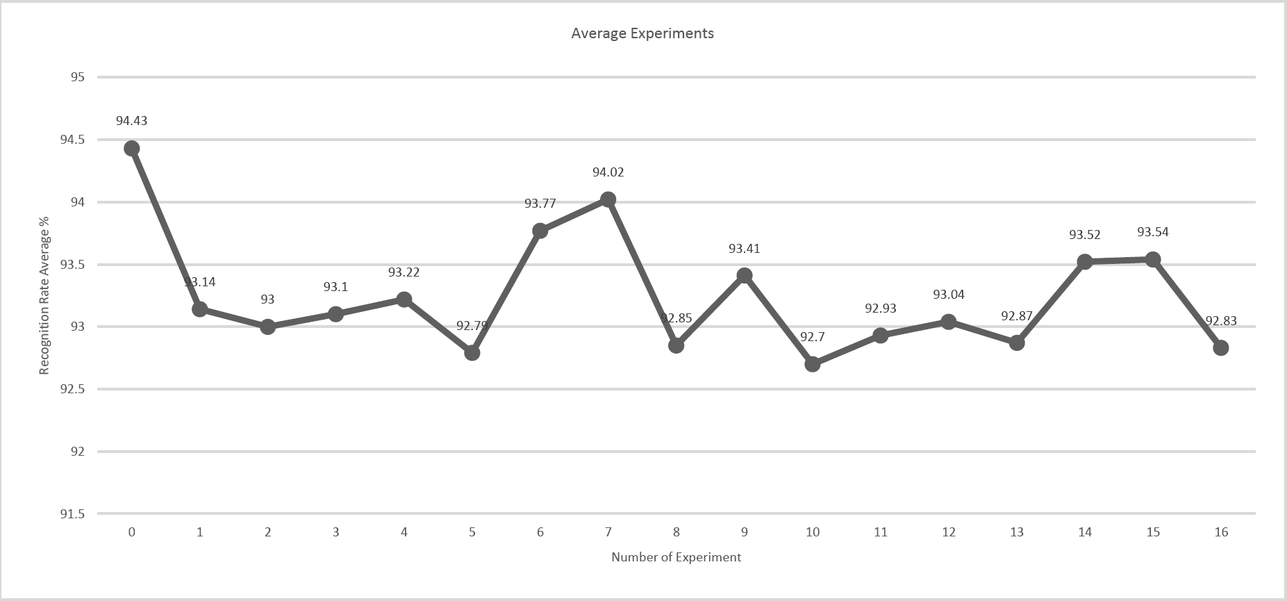
In Table 35 we can see the comparison of the results obtained in the 16 experiments carried out with the experiment zero (0) that refers to the optimization of the filter numbers of the convolution layer 1 and the convolution layer 2 of the convolutional neural network.
Table 35 Comparison of the best results of the experimentation vs the optimization of CNN
| Experiment | EP | Recognition Rate % | NF1 | NF2 |
|
σ | 30 Experiment for each epoch for training |
| 0 | 70 | 97.5 | 15 | 10 | 94.43 | 1.23 | 10,15,20,30,40,50,60,70 |
| 1 | 70 | 95.62 | 25 | 24 | 93.14 | 1.14 | 10,20,30,40,50,60,70,80 |
| 2 | 70 | 95.62 | 25 | 25 | 93 | 1.03 | 40,50,60,70,80 |
| 3 | 80 | 95 | 28 | 30 | 93.10 | 1.23 | 10,20,30,40,50,60,70,80 |
| 4 | 60 | 96.87 | 25 | 27 | 93.22 | 1.24 | 40,50,60,70,80 |
| 5 | 70 | 95.62 | 25 | 25 | 92.79 | 1.25 | 40,50,60,70,80 |
| 6 | 70 | 95.62 | 31 | 31 | 93.77 | 0.99 | 40,50,60,70,80 |
| 7 | 80 | 96.25 | 26 | 27 | 94.02 | 0.89 | 40,50,60,70,80 |
| 8 | 70 | 95.62 | 28 | 28 | 92.85 | 1.23 | 40,50,60,70,80 |
| 9 | 70 | 96.25 | 25 | 27 | 93.41 | 1.30 | 40,50,60,70,80 |
| 10 | 80 | 94.37 | 50 | 50 | 92.70 | 0.88 | 40,50,60,70,80 |
| 11 | 80 | 96.25 | 28 | 28 | 92.93 | 1.22 | 40,50,60,70,80 |
| 12 | 70 | 96.25 | 25 | 18 | 93.04 | 1.14 | 40,50,60,70,80 |
| 13 | 60 | 95 | 24 | 26 | 92.87 | 1.19 | 30,40,50,60,70,80 |
| 14 | 40 | 95.62 | 26 | 16 | 93.52 | 0.93 | 10,20,30,40,50,60,70,80 |
| 15 | 80 | 95.62 | 25 | 27 | 93.54 | 1.12 | 40,50,60,70,80 |
| 16 | 80 | 95 | 25 | 26 | 92.83 | 0.99 | 40,50,60,70,80 |
In Table 36 we can observe the results of the 16 experiments carried out, these results have been ordered from the best average of the obtained recognition percentage to the lowest, also they have been compared with the results of the optimization of the convolutional neural network using the Fuzzy method Gravitational Search Algorithm to find the best number of filters and these results were compared with the best of the experimentation carried out, where a fuzzy system is used where both the inputs and the outputs and their membership functions are triangular or Gaussian and these can be static or dynamic.
Table 36 Comparison of all experiments from highest to lowest of rate recognition average
| Experiment | EP | Recognition Rate % | NF1 | NF2 |
|
σ | 30 Experiment for each epoch for training |
| 0 | 70 | 97.5 | 15 | 10 | 94.43 | 1.23 | 10,15,20,30,40,50,60,70 |
| 7 | 80 | 96.25 | 26 | 27 | 94.02 | 0.89 | 40,50,60,70,80 |
| 6 | 70 | 95.62 | 31 | 31 | 93.77 | 0.99 | 40,50,60,70,80 |
| 15 | 80 | 95.62 | 25 | 27 | 93.54 | 1.12 | 40,50,60,70,80 |
| 14 | 40 | 95.62 | 26 | 16 | 93.52 | 0.93 | 10,20,30,40,50,60,70,80 |
| 9 | 70 | 96.25 | 25 | 27 | 93.41 | 1.30 | 40,50,60,70,80 |
| 4 | 60 | 96.87 | 25 | 27 | 93.22 | 1.24 | 40,50,60,70,80 |
| 1 | 70 | 95.62 | 25 | 24 | 93.14 | 1.14 | 10,20,30,40,50,60,70,80 |
| 3 | 80 | 95 | 28 | 30 | 93.10 | 1.23 | 10,20,30,40,50,60,70,80 |
| 12 | 70 | 96.25 | 25 | 18 | 93.04 | 1.14 | 40,50,60,70,80 |
| 2 | 70 | 95.62 | 25 | 25 | 93 | 1.03 | 40,50,60,70,80 |
| 11 | 80 | 96.25 | 28 | 28 | 92.9375 | 1.22 | 40,50,60,70,80 |
| 13 | 60 | 95 | 24 | 26 | 92.875 | 1.19 | 30,40,50,60,70,80 |
| 8 | 70 | 95.62 | 28 | 28 | 92.85 | 1.23 | 40,50,60,70,80 |
| 16 | 80 | 95 | 25 | 26 | 92.83 | 0.99 | 40,50,60,70,80 |
| 5 | 70 | 95.62 | 25 | 25 | 92.79 | 1.25 | 40,50,60,70,80 |
| 10 | 80 | 94.37 | 50 | 50 | 92.70 | 0.88 | 40,50,60,70,80 |
Comparing the results we can decide that the best results are the experiment number zero (0) which is the optimization of the number of filters of the convolution layers 1 and 2 of the CNN and the second best result obtained (average) is for experiment 8 with a recognition percentage of 94.02% training the network at 80 epochs, using the fuzzy system where the input and the membership functions are Gaussian and dynamic, as well as the outputs that are also Gaussian but with the difference that the Output 1 points are static while Output 2 is not. The third best result of the experiments is experiment number 7, which obtained a recognition percentage of 93.77% with one input and two outputs of the Gaussian and dynamic type fuzzy system. We can see this comparison in detail in Table 37 and in Fig. 4.
Table 37 Details and comparison of all the experiments realized
| Place | Experiment | EP | Recognition Rate % | NF1 | NF2 |
|
σ | 30 Experiment for each epoch for training | Structure of experiment |
| 1 | 1 | 70 | 97.5 | 15 | 10 | 94.43 | 1.23 | 10,15,20,30,40,50,60,70 | FGSA optimizer-C: Conv1 (Opt(15))→ReLU→Pool1→Conv2(Opt (10)) →ReLU→Pool2→Clasif. |
| 2 | 9 | 80 | 96.25 | 26 | 27 | 94.02 | 0.89 | 40,50,60,70,80 | Input: Gaussian Dynamic Output1: Gaussian Static Output2: Gaussian Dynamic |
| 3 | 8 | 70 | 95.62 | 31 | 31 | 93.77 | 0.99 | 40,50,60,70,80 | Input: Gaussian Dynamic Output1: Gaussian Dynamic Output2: Gaussian Dynamic |
In Table 38, we can see the comparison of the CNN optimization (best result obtained so far) with the adaptation of parameters using a fuzzy system where the membership functions change their type (triangular and Gaussian) and their points (dynamic or static).
Table 38 Comparison with other methods
| *Preprocessing Method | Type of network | Optimizat ion / Method | Integrator of response | Recognition rate (%) Max | Recognition rate (%)Max |
Data training | Data tester |
| IT1MGFLS [45] | Modular Neural Network (3 Modules) | No | Sugeno Integral | 97.5 | 88.6 | 80% | 20% |
| IT2MGFLS [45] | Modular Neural Network (3 Modules) | No | Sugeno Integral | 93.75 | 85.98 | 80% | 20% |
| IT1MGFLS [45] | Modular Neural Network (3 Modules) | No | Choquet Integral | 97.5 | 92.59 | 80% | 20% |
| IT2MGFLS [45] | Modular Neural Network (3 Modules | No | Choquet Integral | 97.5 | 91.9 | 80% | 20% |
| Gray and windowing method (4*4) [46] | Artificial neuronal network | No | Not apply | 88.75 | 79.75 | 80% | 20% |
| Gray and windowing method (8*8) [46] | Artificial neuronal network | No | Not apply | 96.25 | 94.25 | 80% | 20% |
| Not apply | Convolutional Neural Network (70 EP)-Optimized with FGSA | FGSA | Not apply | 97.5 | 94.43 | 60% | 40% |
| Not apply | Convolutional Neural Network (80 EP) Optimized with Fuzzy Logic | Fuzzy Logic | Not apply | 96.25 | 94.02 | 60% | 40% |
We can see that although 60% of the images are used for training and 40% for tests and this percentage is much lower than what other methods use, better results are obtained than other works despite using a smaller percentage of images for training. It should be noted that a pre-processing is not being done to the images of the study database; in Fig. 5, we can find the comparison of the data.

Based on the experiments carried out in case study 1 with the ORL database, it was determined that the 3 best methodologies would be taken from all the experiments carried out and they were implemented in 2 more case studies to verify that metaheuristics can also be applied to other case studies.
3.2 Case of Study FERET Database
The FERET database is made up of 111,338 images of human faces, which consists of 994 human faces taken from different angles, 200 images were used to train the neural network (10 images for each human), each image has a size of 256 * 384 pixels in their original size, but a preprocessing of each image was carried out to reduce its size, leaving a final size of 77 * 116 pixels for each image, each one of them is in a .jpg format.
In the following Figure 6 we can see some examples of the original images vs the preprocessed image of the database used.

The first experiment carried out with this database was the optimization of the number of filters using the following architecture for CNN: Arq. Conv1 (Opt) → ReLU → Pool1 → Conv2 (Opt) → ReLU → Pool2 → Classification
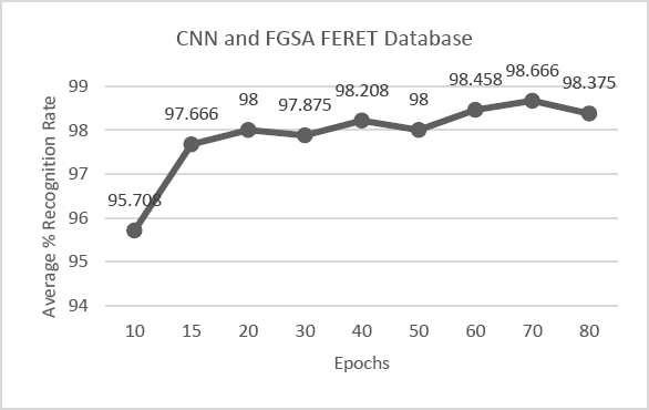
Each experiment was performed 30 times using 15 agents and 3 dimensions in the FGSA, the neural network was trained 10,15, 20, 30, 40, 50, 60, 70 and 80 times, the results obtained show that the best result was 98.66% average in the recognition of the images.
The results can be seen in detail in Table 39, and the results are represented in Fig. 7.
Table 39 Results of first experiment (CNN optimized with FGSA)
| EP | %RR | NF1 | NF2 | σ | |
| 10 | 98.75 | 4 | 3 | 95.70 | 1.34 |
| 15 | 100 | 4 | 2 | 97.66 | 1.07 |
| 20 | 100 | 2 | 1 | 98 | 0.96 |
| 30 | 100 | 7 | 6 | 97.87 | 0.93 |
| 40 | 100 | 7 | 6 | 98.20 | 1.45 |
| 50 | 100 | 9 | 8 | 98 | 1.45 |
| 60 | 100 | 9 | 10 | 98.45 | 0.78 |
| 70 | 100 | 10 | 15 | 98.66 | 1.05 |
| 80 | 100 | 7 | 13 | 98.37 | 1.04 |
The following test is experiment number 7, which is the second-best methodology in which the best results were obtained.
This experiment was carried out applying the proposed method, which, as already mentioned, consists of using the FGSA method for the creation of the membership functions, which are part of the fuzzy system created to find the parameters of the filter numbers of each convolution layer of the neural network.
The membership functions of the input are Gaussian and their values are dynamic, while output 1 has Gaussian and the values are static, unlike output 2, which are Gaussian, but the values are dynamic.
Each output represents the number of filters in each convolution layer of the CNN.
This experiment was carried out 30 times for each training season, the network was trained 40, 50, 60, 70 and 80 times, obtaining the best percentage of recognition of 98.33% with 40 training periods. The results can be seen in Table 40.
Table 40 Results obtained using the methodology of experiment number 7 with the FERET database
| EP | Recognition Rate | NF1 | NF2 | σ | |
| 40 | 100 | 26 | 20 | 98.33 | 1.00 |
| 50 | 100 | 25 | 17 | 98.33 | 1.05 |
| 60 | 100 | 30 | 32 | 98.25 | 1.01 |
| 70 | 100 | 26 | 30 | 98.20 | 0.90 |
| 80 | 100 | 25 | 18 | 98.12 | 0.97 |
The third methodology with the best results was experiment #6, which uses membership functions of the input: Gaussian and Dynamic. In the same way, the 2 outputs of the fuzzy system are Gaussian and dynamic. This experiment was performed 30 times for each training season and the CNN was trained 40, 50, 60, 70 and 80 times, obtaining an average 98.20% as the best recognition result and 100% with its maximum percentage in the recognition of the images from the FERET database when the network is trained 70 times.
In Table 41, we can find the obtained results.
Table 41 Results obtained using the methodology of experiment number 6 with the FERET database
| EP | Recognition Rate | NF1 | NF2 | σ | |
| 40 | 100 | 30 | 30 | 98.12 | 1.02 |
| 50 | 100 | 30 | 27 | 98.08 | 1.17 |
| 60 | 98.75 | 26 | 23 | 98 | 0.77 |
| 70 | 100 | 32 | 20 | 98.20 | 0.84 |
| 80 | 100 | 16 | 17 | 98 | 0.77 |
In Table 42, we have the compilation of the best results obtained, in which we can verify that the best result in the recognition of the images is when the CNN is optimized, following the proposed method with the methodology of experiment # 7 and finally in third place was experiment # 6.
Table 42 Results comparative with experiments FERET database
| Experiment | EP | Recognition Rate % | NF1 | NF2 |
|
σ | 30 Experiment for each epoch for training | Structure of experiment |
| 1 | 70 | 100 | 10 | 15 | 98.66 | 1.04 | 10,15,20,30,40,50,60,70,80 | FGSA optimizer-C: Conv1 (Opt(10))→ReLU→Pool1→Conv2(Opt (15)) →ReLU→Pool2→Clasif. |
| 9 | 40 | 100 | 26 | 20 | 98.33 | 1.00 | 40,50,60,70,80 | Input: Gaussian Dynamic Output1: Gaussian Static Output2: Gaussian Dynamic |
| 8 | 70 | 100 | 32 | 20 | 98.20 | 0.84 | 40,50,60,70,80 | Input: Gaussian Dynamic Output1: Gaussian Dynamic Output2: Gaussian Dynamic |
The results obtained were compared with different methodologies, where we can see that the results obtained, both optimizing the network and introducing the proposed method, obtain better results than the rest of the compared methods, we can observe in Table 43.
Table 43 Results comparative with experiments FERET database with other methods and neural networks
| Preprocessing Method | Type of network | Optimization | Integrator of response | Average recognition rate (%) | Recognition rate (%) | σ | Data training | Data tester |
| T1 FSs [47] | Monolithic neural network. | No | Sobel +T1 FSs | 82.77 | 83.78 | 0.68 | 80% | 20% |
| IT2 FSs [47] | monolithic neural network | No | Sobel + IT2 FSs | 84.46 | 87.84 | 0.32 | 80% | 20% |
| GT2 FSs [47] | monolithic neural network | No | Sobel + GT2 FSs | 87.50 | 92.50 | 0.08 | 80% | 20% |
| Not Applied | Canonical Correla3tion Analysis (CCA) [48] | No | Not applied | - | 40% | - | - | |
| Not Applied | Linear Discriminant Analysis (LDA) [48] | No | Not applied | - | 95% | - | - | |
| Viola-Jones algorithm, Resize 100*100 [49] | MNN | Grey Wolf Optimizer | - | 92.63% | 98% | 4.05 | up to 80% | 20% |
| Not applied | Convolutional Neural Network (70 EP) Optimized with FGSA | FGSA | Not applied | 98.66 | 100% | 1.04 | 60% | 40% |
| Not applied | Convolutional Neural Network (40 EP) Optimized with Fuzzy Logic | Fuzzy Logic | Not applied | 98.33 | 100% | 1.00 | 60% | 40% |
3.3 Case of Study MNIST database
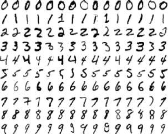
The third case study selected to use the proposed methodologies is the MNIST database, which consists of handwritten numbers, it consists of 60,000 images and has a set of 10,000 images for testing, we use the set of test images of 10,000 images which each image has a size of 28 * 28 pixels in black and white, 60% of images were used for training and 40% for tests.
For this case study we use 2 different architectures for the convolutional neural network, which are the following:
1- Arq. Conv1 (Opt) → ReLU → Pool1 → Conv2 (Opt) → ReLU → Pool2 → Classif.
2- Arch. Conv1 (Opt) → ReLU → Pool1 → Conv2 (Opt) → ReLU → Pool2 → Conv3 (Opt) → ReLU → Pool3 → Classification
In the first architecture there are 2 convolution layers and two pooling layers, while in the second architecture 1 convolution layer was added, as well as a pooling layer to the architecture, thus deepening the neural network to improve the recognition percentage in the images.
In Figure 8 we can find some of the images that make up the MNIST database.
In experiment # 0, which deals with the optimization of the number of CNN filters, architecture # 1 was used, in which an exhaustive experimentation was carried out, carrying out 30 times each training period, until obtaining the best result for this architecture. In this case, the network was trained 10000 times resulting in an average 86.19% and a maximum of 87.47% in image recognition and the number of filters of each convolution layer was 57 and 73 respectively.
In Table 44 we can find a summary of the best results for each training season in which this case study was experimented.
Table 44 Results obtained with the experiment #1 using the Architecture #1
| EP | %RR | NF1 | NF2 | σ | |
| 10 | 84.21 | 1 | 9 | 81.51 | 1.25 |
| 15 | 84.63 | 15 | 10 | 83.16 | 0.86 |
| 20 | 85.93 | 8 | 14 | 82.89 | 0.72 |
| 30 | 86.04 | 8 | 12 | 84.61 | 0.76 |
| 40 | 87.62 | 11 | 12 | 85.15 | 0.90 |
| 50 | 86.94 | 7 | 10 | 85.24 | 0.79 |
| 60 | 87.11 | 12 | 7 | 85.10 | 1.00 |
| 70 | 87.54 | 7 | 6 | 85.12 | 0.95 |
| 80 | 86.86 | 6 | 5 | 84.92 | 0.81 |
| 90 | 86.91 | 14 | 2 | 85.18 | 0.77 |
| 100 | 88.08 | 2 | 11 | 85.29 | 0.93 |
| 150 | 87.48 | 10 | 10 | 85.41 | 0.89 |
| 200 | 86.78 | 12 | 7 | 85.44 | 0.73 |
| 300 | 86.39 | 6 | 5 | 85.20 | 0.61 |
| 400 | 86.68 | 9 | 14 | 85.22 | 0.69 |
| 500 | 86.88 | 97 | 83 | 85.73 | 0.71 |
| 700 | 86.87 | 40 | 42 | 85.73 | 0.62 |
| 1000 | 88.04 | 46 | 40 | 85.82 | 0.77 |
| 3000 | 84.21 | 57 | 47 | 85.88 | 0.67 |
| 6000 | 88.84 | 19 | 17 | 86.14 | 0.92 |
| 10000 | 87.47 | 57 | 73 | 86.19 | 0.63 |
The FGSA method with the following parameters were used for all experiments in which this method was used, 15 agents with 3 dimensions.
In experiment # 7, 30 iterations were carried out for each time and the network was trained 10,000, 6,000, 3,000 and 1,000 times, obtaining the best result when the CNN is trained with 10,000 times with a maximum of 86.49% and an average of 86.11. image recognition. In Table 45 we can find each result in detail.
Table 45 Results obtained with experiment #7 using Architecture #1
| EP | %RR | NF1 | NF2 | σ | |
| 10000 | 86.49 | 67 | 63 | 86.11 | 0.64 |
| 6000 | 88.64 | 39 | 43 | 86.10 | 0.89 |
| 3000 | 86.68 | 44 | 47 | 85.89 | 0.63 |
| 1000 | 87.09 | 56 | 43 | 85.41 | 0.79 |
Table 46 presents the results obtained in experiment # 6, which occupies the third place of the methodologies that yielded the best result based on the experimentation of case study # 1, this experiment consisted in training the neural network with 10000,6000 and 3000 epochs, 30 times for each case, and we observe that the maximum value is 86.88% and an average of 83.19% in the recognition of the images.
Table 46 Results obtained with experiment #6 using Architecture #1
| EP | %RR | NF1 | NF2 | σ | |
| 10000 | 86.88 | 45 | 73 | 83.19 | 0.63 |
| 6000 | 88.09 | 41 | 54 | 83.10 | 0.78 |
| 3000 | 86.76 | 15 | 87 | 82.78 | 0.63 |
Based on previous experiments with the CNN architecture # 1, it was decided to deepen the network further, adding a convolution layer and a pooling layer to the architecture to find out if this new architecture could obtain better results.
Table 47 shows the results in which architecture # 2 was applied, where the network was trained 100, 500, 1000 and 5000 epochs each with 30 iterations respectively. In this experiment, experiment # 0 was applied in which the network is optimized using the FGSA method, the results show that the best recognition value obtained was 91.18% and with an average of 89.82% in the recognition of the images with this case study with 1000 epochs training. The number of filters for the convolutional layer 3 is called NF3.
Table 47 Results obtained with the experiment #7 using the Architecture #1
| EP | Recognition Rate | NF1 | NF2 | NF3 | σ | |
| 100 | 91.33 | 61 | 66 | 18 | 89.72 | 0.60 |
| 500 | 91.29 | 61 | 66 | 18 | 89.80 | 0.59 |
| 1000 | 91.18 | 61 | 66 | 18 | 89.82 | 0.57 |
| 5000 | 90.70 | 10 | 4 | 33 | 89.78 | 0.54 |
In Table 48, we can find the compilation of the best results obtained with architecture # 1 and the Table 49 the architecture # 2. Based on the previous experimentation, it was decided not to test the proposed method for architecture 2 since the increase in image recognition is minimal and it is more time and computing resource consuming.
Table 48 Comparative results for the MNIST database with architecture #1 using the experiment #0
| Arq. Conv1 (Opt)→ReLU→Pool1→Conv2(Opt) →ReLU→Pool2→Clasif | ||||||||
| Experiment | EP | %RR | NF1 | NF2 |
|
σ | 30 Experiment for each epoch for training | Structure of experiment |
| 0 | 10000 | 87.47 | 57 | 73 | 86.19 | 0.63 | 10000,6000,3000,1000,700,500,400,300,200, 150,100,90,80,70,60,50,40,30,20,15,10 | FGSA optimizer-C: Conv1 (Opt(57))→ReLU→Pool1→Conv2(Opt (73)) →ReLU→Pool2→Clasif. |
| 7 | 10000 | 86.49 | 67 | 63 | 86.11 | 0.64 | 10000,6000,3000,1000 | Input: Gaussian Dynamic Output1: Gaussian Static Output2: Gaussian Dynamic |
| 6 | 10000 | 86.88 | 45 | 73 | 83.19 | 0.63 | 10000,6000,3000,1000 | Input: Gaussian Dynamic Output1: Gaussian Dynamic Output2: Gaussian Dynamic |
4 Conclusions
As final conclusions of this experimentation, it has been observed that the optimization of the convolutional neural network with the number of filters using the FGSA method yields better results than with the proposed method using a fuzzy system, which is in charge of finding the best values for the parameters of the number of filters of each convolution of the network.
Another observation we have is that although the difference between the optimization and the proposed method is minimal, providing similar values, but nonetheless not better than using a bio-inspired algorithm to optimize the network as is the case of the Fuzzy Gravitational Search Algorithm method.
It was also observed that although the depth of the network is increased, better results are not always obtained and this depends on the database that is being used, the more complex it is, the deeper it is to extract more main characteristics; therefore, the simpler case study will be the CNN architecture and therefore the resources to use both in time and computing will also be less.
It was observed that the Gaussian-type membership functions produced better results than the triangular membership functions for the most part when these were dynamic rather than static.
As future work, more experimentation with the method will be carried out, modifying the depth of the convolutional neural network as well as making use of other more complicated databases to observe and analyze the data obtained. Based on the results obtained with type-1 fuzzy logic, it is intended as future work to implement type-2 fuzzy logic in the best architectures obtained in the work. It is expected to significantly improve the results obtained using this methodology and tested in new and more complicated databases.

