


 text new page (beta)
 English (pdf)
 Article in xml format
 Article references
 Send this article by e-mail
 Cited by SciELO
  Similars in
SciELO
Similars in
SciELO 
 Permalink
1 Introduction
Mobile robot navigation includes all the actions that lead a robot to move from its current position to its destination [2, 5]. Path planning is an essential navigation task that generates a collision-free trajectory that a robot follows during its movement [5]. The fuzzy inference systems (FIS) [7, 15], the artificial potential fields (APF) [9], reinforcement learning (RL) [6, 11, 18], and the neuronal networks (NN) [10, 19] are some of the considered approaches for robot navigation demonstrating advantages and disadvantages.
An attractive path planning method is the APF, thanks to its simplicity and low computational cost demands [9].
Researchers rely on and use these methods [1] to complete the navigation tasks for path planning and obstacle avoidance. However, to prevent a sudden robot's shutdown, it is also essential to propose a solution considering that the battery charge level tends to run out during regular execution tasks. This issue is known as the autonomous recharging problem (ARP) [4].
The ARP arises due to the importance of mobile robots to have autonomy and self-sufficiency when using batteries. Hence, suitable strategies must be chosen to allow these robots to function for as long as possible.
The more straightforward approach consists of placing a threshold allowing the robot's task execution while the battery level is above the threshold. If the battery level is below the threshold, the robot leaves its programmed task to recharge the batteries.
However, this strategy induces inflexible and inefficient robot behavior [17]. With this in mind, the following question arises, how could a robot learn to select actions to complete its task autonomously and at the same time to cope with the ARP? One of several solutions consists of making the robot learn based on tests and errors.
To this end, this paper presents a learning technique for the robot's action selection combined with a reinforcement learning paradigm.
The proposed navigation technique consists of a module for path planning using APF and a second module for decision-making, including an architecture based on Fuzzy Q-Learning (FQL) to select when to go to a charging station.
The rest of the paper is organized as follows. Section 2 describes the related works, while section 3 is focused on presenting the theoretical concepts related to the proposed methods. Section 4 is oriented to define the problem statement, while section 5 is focused on explaining the proposal. Section 6 shows the simulation results, while section 7 is dedicated to present the discussions. Finally, in section 8, the conclusions are enumerated.
2 Related Work
Among the sub-tasks that are part of any mobile robot navigation system are obstacle avoidance, path planning, and decision-making. In this work, we focus on decision-making. Therefore, the related work shows below talks about the ARP. If the robot does not recharge its batteries, it could shut down before completing its tasks.
A simple strategy to solve this problem is to place a threshold that makes the robot a little flexible. As in Rappaport's work, some approaches use this philosophy [13] that selects an adaptative threshold to choose a charging station to go to when the battery level is below that threshold. On the other hand, Cheng [3] proposes a strategy based on an algorithm to program the minimum time of meetings between mobile robots and mobile chargers.
This strategy consists of having a series of mobile battery recharging stations, which the robots look for every so often to recharge their batteries. Similarly, Ma [12] proposes to work with time windows and focuses on the recharging of autonomous vehicles. The proposal considers the charging station's capacity and the delays in the queue for recharging vehicles. Meanwhile, Tomy [17] also manages a recharge program, and he uses Markov models, which provides his proposal with a dynamic behavior based on the environment and a reward system. Another strategy used to solve the problem is a rule-based strategy thanks to a FIS, which allows the robot to have flexibility according to the inputs, as can be seen in Lucca's [4] work.
A point noted in previous work is the lack of learning algorithms that allow robotic systems to learn when to recharge their batteries. For that reason, this work faces that problem with the use of reinforcement learning.
3 Preliminaries
This section summarizes the methods analyzed and used in this work for path planning; first, the APF method is described and ends with the FQL method description used in the decision-making module.
3.1 The Artificial Potential Field Method
This method is based on attractive and repulsive forces that are used to reach a goal and avoid obstacles. Equation (1) computes the attractive force, where 𝜉 is the attractive factor, 𝜌(𝑞, 𝑔) is the euclidean distance between the robot and the goal, 𝑞 is the robot position, and 𝑔 its goal position:
The expressions shown in equation (2) are used to compute the repulsive force, where η is the repulsive factor,
Finally, the resultant force (3) is the sum of attractive and repulsive forces:
3.2 Fuzzy Q-Learning Method
FQL method [8] is an extension of the FIS. The method starts with the fuzzification of the inputs to obtain the fuzzy values identifying the system's current fuzzy rule
The learning agent's goal is to find the action with the best q-value, which is stored on a table containing
where
The inferred action 𝑎(𝑥) and the q-value 𝑄(𝑥, 𝑎) are computed given the equation in (5) and (6), respectively:
where 𝑖𝑜 is the inferred action index, and 𝑁 is a positive number 𝑁 ∈ 𝑁+, that corresponds to the total number of the rules.
On the other hand, to update the q-value, in the table, is used an eligibility value 𝑒(𝑖, 𝑗).
That is rendered from an array of 𝑖 × 𝑗 values; usually, this array is initialized with zeros. The 𝑒(𝑖, 𝑗) value is updated employing equation (7), where 𝑗 is the selected action, γ is the discount factor 0 ≤ γ ≤ 1, and 𝜆 is the decay parameter 𝜆 ∈ [0,):
Finally, equation (8) allows updating the q-value, where 𝜖 is a small number
where 𝑟 corresponds to the reward.
4 Problem Statement
The problem addressed in this paper is focused on learning to select between moving on to the destination or going to recharge the batteries. For this purpose, a robot is considered in a static environment with twenty scattered obstacles in a 10 × 10 grid. The robot must move without collision from a starting point to a destination. According to its battery level, the robot must decide whether to continue to the destination or detour to recharge it. The robot can move forward, backward, left or right.
Four main elements are considered in this research: (1) A robot denoted as 𝑅, (2) 𝑁 obstacles denoted as 𝑂 = [𝑂1, 𝑂2, . . . , 𝑂𝑁], and 𝑁 ∈ [1,20], (3) The destination denoted as 𝐷, and (4) A battery charging station denoted as 𝐵𝐶𝑆.
The robot can execute two actions denoted as 𝐴 = [𝑎1, 𝑎2], where 𝑎1 corresponds to the action go to 𝐷, and 𝑎2 is going to the 𝐵𝐶𝑆.
Elements 2, 3, and 4 are static, where the 𝑂, 𝐷, and 𝐵𝐶𝑆 do not change their position concerning time. The robot uses a coordinate map of 10 × 10 dimensions. At the beginning, the robot knows the position of 𝐷 and 𝐵𝐶𝑆 and uses a path planning module to generate a route to 𝐷 and other to 𝐵𝐶𝑆.
Figure 1 shows the discharge curve with the voltage levels and percentage of charge of a Li-Po 11.1v battery for the robot battery simulation [15].
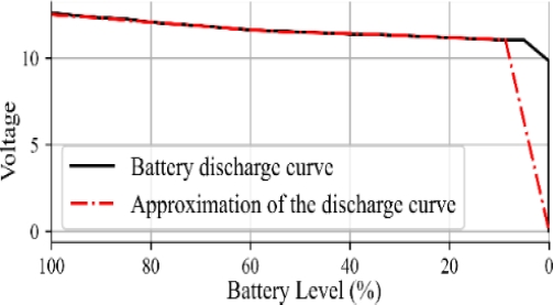
The equation 𝐵𝐿(𝑡) = −1.8245𝑡 + 100 , where 𝐵𝐿 corresponds to the battery level, serves to approximate this discharge curve, and Figure 1 shows this approximation with a dash and dot line.
At each step, the robot calculates the Euclidean distance of its position to 𝐷 and BCS. The distances calculated at the beginning are IDC, the initial distance between the R and BCS, and 𝐼𝐷𝐷 the initial distance to 𝐷.
Simultaneously, the distances calculated in each step are CDD, the current distance to D, and 𝐶𝐷𝐶 the current distance to the 𝐵𝐶𝑆:
The function 𝐷𝑅𝐷 in (10) is used to normalize the current distance to the 𝐷, while the function 𝐷𝑅𝐶 in (11) is used to normalize the distance to the 𝐵𝐶𝑆:
5 Navigation Approach
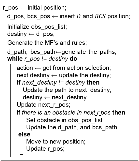
Algorithm 1 is proposed to handle the course of a robot so that it can navigate in a scenario with static obstacles, integrating a path planning module and a rule-based RL approach with FQL to select the action to be executed by the robot.
5.1 Path planning
The path planning module conducted with the APF uses the equations shown in section 3. The selection of the attractive and repulsive factors (𝜉 = 2.3 , and 𝜂 = 61.5) was implemented, employing a differential evolution algorithm [14] with interval values in [0,100].
Algorithm 2 shows the procedure followed to generate a path, where the entries are the R position and the D's position. This algorithm runs twice at starting to generate a path for going to the D and going to the 𝐵𝐶𝑆.

5.2 Action Selection
The proposal for action selection consists of three inputs and two possible outputs. These inputs are BL, CDD, and CDC. The outputs are associated with a numerical value used to define which action to select, the action with the highest numerical value is chosen.
In the same way that FIS uses membership functions (MF), this architecture occupies the MFs shown in Figure 2. The MF of the BL input has three fuzzy sets that correspond to the level of the battery full (FB), low (LB), and very low (VLB); the MFs of the CDD and CDC inputs have fuzzy sets far (F), near (N), and very near (C).

Using the three proposed entries with their corresponding MFs, this system has the twenty-seven fuzzy rules shown in Table 1, where the output can be 𝑎1 or 𝑎2 depending on the computed q-values.
Table 1 Fuzzy rules
| Rule | BL | CDD | CDC | Output |
| 1 | VLB | C | C | action=𝑎1|𝑎2 |
| 2 | VLB | C | N | action=𝑎1|𝑎2 |
| 3 | VLB | C | F | action=𝑎1|𝑎2 |
| 4 | VLB | N | C | action=𝑎1|𝑎2 |
| 5 | VLB | N | N | action=𝑎1|𝑎2 |
| 6 | VLB | N | F | action=𝑎1|𝑎2 |
| 7 | VLB | F | C | action=𝑎1|𝑎2 |
| 8 | VLB | F | N | action=𝑎1|𝑎2 |
| 9 | VLB | F | F | action=𝑎1|𝑎2 |
| 10 | LB | C | C | action=𝑎1|𝑎2 |
| 11 | LB | C | N | action=𝑎1|𝑎2 |
| 12 | LB | C | F | action=𝑎1|𝑎2 |
| 13 | LB | N | C | action=𝑎1|𝑎2 |
| 14 | LB | N | N | action=𝑎1|𝑎2 |
| 15 | LB | N | F | action=𝑎1|𝑎2 |
| 16 | LB | F | C | action=𝑎1|𝑎2 |
| 17 | LB | F | N | action=𝑎1|𝑎2 |
| 18 | LB | F | F | action=𝑎1|𝑎2 |
| 19 | FB | C | C | action=𝑎1|𝑎2 |
| 20 | FB | C | N | action=𝑎1|𝑎2 |
| 21 | FB | C | F | action=𝑎1|𝑎2 |
| 22 | FB | N | C | action=𝑎1|𝑎2 |
| 23 | FB | N | N | action=𝑎1|𝑎2 |
| 24 | FB | N | F | action=𝑎1|𝑎2 |
| 25 | FB | F | C | action=𝑎1|𝑎2 |
| 26 | FB | F | N | action=𝑎1|𝑎2 |
| 27 | FB | F | F | action=𝑎1|𝑎2 |
To calculate the numerical value for actions 𝑎1 and 𝑎2, we can use the equations given in section 3 as it is shown in Algorithm 3. On the other hand, 𝛼 is equal to 0.01, and 𝛾 is equal to 0.9. these values were selected after obtaining a faster learning rate than other tested values.

The method starts with a table of q values equal to zero. The update of the q-values occupies the reward function defined in equation (12):
6 Simulation Results
Simulations constrain the R's movement on a 10 × 10 grid, where the R can move forward, right, left, and backward. The initial position of the R starts at the coordinates (0,0) of the grid, 𝐷 is at (5, 9), and 𝐵𝐶𝑆 is at (9,5). Given the MFs shown in Figure 2, this section shows the simulations in fifteen scenarios tested. For experimentation, the battery behavior is simulated using the expression BL(t), described in section 4, where t corresponds to a time step, and so, every step execution, the battery level decrease accordingly to expression BL(t). Alternatively, increase every time the R reaches BCS. The current BL can replace this arrangement during implementation in a real robot. The navigation proposal trained until completing five successful trajectories to the 𝐷.
The following tables show a comparison between the QL method and a FIS, while the figures illustrate the behavior of the proposal presented in this paper. QL method uses the same learning rate, discount factor, and reward function used for our proposal. Like the proposed FQL method, QL and FIS methods use the three inputs corresponding to the BL, CDC, and CDD.
Figure 3 shows the total epochs taken in each scenario. In two scenarios, the number of epochs to complete the trajectory was higher than in the others. It means that for these two scenarios, the R spent more time deciding which actions to execute to complete the path to the D. However, in Table 2, it is observed that the number of epochs our proposal takes is smaller in comparison with the QL method, which is advantageous because the time it took the R to select and execute the actions was reduced. Note that since the FIS method does not have learning, this variable does not apply, so it is denoted as NA in the table.

Fig. 3 Number of epochs it took the simulation to complete the trajectory successfully five times in fifteen scenarios
Table 2 Number of epochs it took for the simulation to complete the trajectory successfully five times with the FQL proposal and QL method
| Scenarios | FIS | QL | FQL |
| 1 | NA | 17 | 5 |
| 2 | NA | 23 | 6 |
| 3 | NA | 22 | 5 |
| 4 | NA | 13 | 5 |
| 5 | NA | 166 | 5 |
| 6 | NA | 22 | 67 |
| 7 | NA | 59 | 5 |
| 8 | NA | 25 | 10 |
| 9 | NA | 13 | 5 |
| 10 | NA | 110 | 5 |
| 11 | NA | 33 | 71 |
| 12 | NA | 80 | 10 |
| 13 | NA | 39 | 5 |
| 14 | NA | 17 | 8 |
| 15 | NA | 24 | 5 |
Figure 4 shows the BL and the number of steps obtained in one of the epochs where the R completed its trajectory in each scenario using the FQL method.

Fig. 4 Battery level and the number of steps with which the robot completed each of the proposed scenarios
According to the observed results, the BL with which the R completed the trajectory was above 70% in most scenarios. Likewise, the number of steps executed remained below 20. Table 3 shows that the BL value at the end of each scenario is very close to the BL at the end of the FIS; contrarily to the QL method, there were five cases where the BL was inferior to 50%, showing that our proposal performs better compared to QL method. Nevertheless, Table 3 also shows that the FIS ended the simulation with the highest BL in almost all cases. This behavior is because, with the FIS, there were no deviations towards the BCS, and the simulated R went straight to D, contrary to the case of the FQL and QL methods. However, the results show that the FQL method learns to select the actions that help it finish with a BL similar to the FIS method.
Table 3 The battery level at which the simulation ended using FIS, QL, and FQL methods in each scenario during the fifth completed trajectory
| Scenarios | FIS | QL | FQL |
| 1 | 78.0 | 51.0 | 74.4 |
| 2 | 78.0 | 65.0 | 67.1 |
| 3 | 74.4 | 65.0 | 74.4 |
| 4 | 78.0 | 76.0 | 78.0 |
| 5 | 78.0 | 40.0 | 78.0 |
| 6 | 78.0 | 14.0 | 78.0 |
| 7 | 74.4 | 80.0 | 70.7 |
| 8 | 78.0 | 69.0 | 78.0 |
| 9 | 78.0 | 73.0 | 78.0 |
| 10 | 78.0 | 32.0 | 67.1 |
| 11 | 70.1 | 80.0 | 70.7 |
| 12 | 78.0 | 47.0 | 78.0 |
| 13 | 78.0 | 40.0 | 74.4 |
| 14 | 78.0 | 73.0 | 74.4 |
| 15 | 78.0 | 58.0 | 78.0 |
Additionally, in the graph presented in Figure 5, the R sometimes selected action 𝑎2 which caused a route change towards the BCS. Under whose test conditions, in most cases, the R selected the action of going to the 𝐷, meaning that the number of steps to D could have been less, however during the action selection, the R decides that it has to charge the battery and deviates from the original route. The executed steps varied between two and six compared to those that the FIS method executed, as shown in Table 4, whose the executed steps were between 14 and 18 according to the scenario.

Fig. 5. of times that the actions 𝑎1 and 𝑎2 were selected during the displacement to the destination
Table 4 The number of steps at which the simulation ended using FIS, QL, and FQL methods in each scenario during the fifth completed trajectory
| Scenarios | FIS | QL | FQL |
| 1 | 14 | 30 | 16 |
| 2 | 14 | 22 | 20 |
| 3 | 16 | 22 | 16 |
| 4 | 14 | 16 | 14 |
| 5 | 14 | 36 | 14 |
| 6 | 14 | 50 | 14 |
| 7 | 16 | 14 | 18 |
| 8 | 14 | 20 | 14 |
| 9 | 14 | 18 | 14 |
| 10 | 14 | 40 | 20 |
| 11 | 18 | 14 | 18 |
| 12 | 14 | 32 | 14 |
| 13 | 14 | 36 | 16 |
| 14 | 14 | 18 | 16 |
| 15 | 14 | 26 | 14 |
The FIS, being a rule-based method and lacking any learning stage, completes the task with the fewest number of steps executed. Whereas methods that have to learn to select actions that help to complete the task execute more steps. According to Table 4 results, the proposed FQL method completes the task in a minor sequence of steps than QL method.
The breakdown of the actions selected in each scenario is depicted in Table 5. The results show that the simulated R always selects to go towards D using the FIS method. Unlike QL and FQL methods, which in some cases selected action 𝑎2 causing the simulated R to divert towards the BCS instead of going towards D, and therefore, it caused that they took longer to get to D than the FIS method.
Table 5 The number of times actions 𝑎1 and 𝑎2 were selected during the simulation
| Scenario | Action | Method | ||
| FIS | QL | FQL | ||
| 1 | 𝑎1 | 14 | 20 | 9 |
| 𝑎2 | 0 | 10 | 7 | |
| 2 | 𝑎1 | 14 | 12 | 16 |
| 𝑎2 | 0 | 10 | 4 | |
| 3 | 𝑎1 | 16 | 12 | 13 |
| 𝑎2 | 0 | 10 | 3 | |
| 4 | 𝑎1 | 14 | 9 | 13 |
| 𝑎2 | 0 | 7 | 1 | |
| 5 | 𝑎1 | 14 | 23 | 10 |
| 𝑎2 | 0 | 13 | 4 | |
| 6 | 𝑎1 | 14 | 27 | 10 |
| 𝑎2 | 0 | 23 | 4 | |
| 7 | 𝑎1 | 16 | 10 | 12 |
| 𝑎2 | 0 | 4 | 6 | |
| 8 | 𝑎1 | 14 | 12 | 11 |
| 𝑎2 | 0 | 8 | 3 | |
| 9 | 𝑎1 | 14 | 12 | 12 |
| 𝑎2 | 0 | 6 | 2 | |
| 10 | 𝑎1 | 14 | 21 | 15 |
| 𝑎2 | 0 | 19 | 5 | |
| 11 | 𝑎1 | 18 | 10 | 16 |
| 𝑎2 | 0 | 4 | 2 | |
| 12 | 𝑎1 | 14 | 20 | 7 |
| 𝑎2 | 0 | 12 | 7 | |
| 13 | 𝑎1 | 14 | 20 | 12 |
| 𝑎2 | 0 | 16 | 4 | |
| 14 | 𝑎1 | 14 | 10 | 12 |
| 𝑎2 | 0 | 8 | 4 | |
| 15 | 𝑎1 | 14 | 12 | 10 |
| 𝑎2 | 0 | 14 | 4 | |
Furthermore, Figure 6 shows the accumulated reward. When the training lasted longer, the accumulated reward rises because the R was moving towards the 𝐵𝐶𝑆. While the number of steps to complete the trajectory was minor in the scenarios, the reward remained below 50.

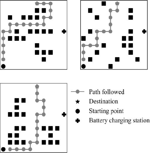
Finally, Figure 7 shows a sample of three of the fifteen scenarios in which the tests were carried out. The graphs in this figure are composed of five elements:
1. The squares represent the obstacles,
2. The cross corresponds to the position of the BCS,
3. The star positions the D
4. The circle represents the starting point of the R
5. The line with circles is the trajectory followed by R.
7 Discussion
During simulations, the obstacles used in scenarios were placed in different positions. The variations of the path generated with the path planning method affected the task performance reflected in the number of steps invested by the system to complete the path to 𝐷. During training, when the robot was close to the 𝐵𝐶𝑆, and the BL was different from BF, the robot followed the 𝐵𝐶𝑆 path instead of 𝐷, and it remained there.
So, the robot failed to complete its task to go to 𝐷. With this approach, an expert can define the number of states that the agent takes, as in a traditional FIS. With the addition that the system can learn based on trial and error using QL method. Comparing our proposal with the traditional QL method, the number of states that the agent can take is reduced to the number of rules that the expert defines. To visualize this, take the example of the battery level input.
In QL method, the number of states that the agent can take ranges from 0 to 100, while with this proposal, there are 27 states, which helps to reduce computational complexity. By adding the distances to D and 𝐵𝐶𝑆 as inputs, the number of states would grow even more until 1,030,301. Among the disadvantages, the system might not necessarily choose the shortest path at all times, since in some steps, the learning agent may select to remain in standby mode. However, with the acquired learning, the system manages to select the actions that allow it to complete its task.
8 Conclusions
The proposed navigation technique demonstrates the robot's capability of duly selecting any of the actions 𝑎1 and 𝑎2, which allows it to fulfill its goal to reach a predetermined destination maintaining the battery charge level in appropriate condition, based on a decision-making methodology.
Using the FQL method, the number of defined rules assigns the system's complexity, unlike the classical QL method, where the states would correspond to possible battery level measurements. The proposed methodology limits the number of states to the ranges assigned with the MFs and helps a robot learns to select tasks autonomously and complete its task.
In this paper's case, the assigned tasks were the displacement to some destination D or BCS. The simulated robot reached the D successfully, although sometimes, the robot took a deviation to the BCS to maintain its battery in conditions to finish the started task.
However, whether other functions are added to the list of tasks, like taking a bottle, it will be necessary to consider the task time execution and the discharge battery curve to guarantee that the robot will select the best action to maintain itself working and finish the started job successfully.
For future work, we propose to study how to integrate this functionality in the proposed algorithms to guarantee success with any assigned task and test the proposal in realistic scenarios.
This approach, compared to a traditional QL method or a FIS, has certain advantages. Unlike the FIS method, in an FQL, an expert does not need to assign the output to be executed since the proposal made with the FQL allows a robot to learn autonomously to select actions. According to the results presented, the proposal can match the results of a FIS during the decision-making process since the battery levels and the number of steps with which the simulations ended were similar in most of the scenarios tested. While it dramatically improves the results obtained with the QL method. Besides, it significantly reduces the number of states. Consequently, it reduces the among of memory occupied for learning, which will allow the implementation of the proposal in a robot with low computing capabilities.

