


 text new page (beta)
 English (pdf)
 Article in xml format
 Article references
 Send this article by e-mail
 Cited by SciELO
  Similars in
SciELO
Similars in
SciELO 
 Permalink
1 Introduction
There are many multidisciplinary fields, in which the classification problems are important. Currently, there are several classifiers reported in literature. These classifiers are based on different concepts as neuronal networks, Bayesian networks, classification trees, logistical regression or discriminant analysis.
In fields like Bioinformatics, it is not possible to solve complex problems in a satisfactory way with the use of a single classifier. Frequently, in these fields the metric (precision, accuracy or error) of one only classifier does not satisfy the problem requirements. This is the main reason that has lead the use of systems of several classifiers to try to reach superior results regard an only classifier.
Many authors use the term "classifier ensemble", as a "classifier" that combines the outputs of a set of individual classifiers, using some approach (e.g.: average, majority vote, minimum, etc.). These classifier ensembles are able to satisfy many times the necessity to develop exact, precise and reliable classifiers for many practical applications. There are many reported articles that use classifier ensembles with success in the solution of real problems [1-3]. The idea to combine individual classifiers begins of the fact of combining complementary answers.
The classifiers that should combine are not the most precise or the most exact, are the most diverse. If the classifiers are diverse then an example (instance) incorrectly classified by one or several classifiers can be correctly classified by others [4].
The combination of identical classifiers not produce better results. The main idea is combine a set of diverse classifiers to each other, to guarantee that at least one of them offers the correct answer when the rest is mistaken. For this reason, it is extremely important study the diversity among the individual classifiers to combine.
The diversity should be considered as a guide during the process of design of a classifier ensemble. In this process an main objective is the inclusion of individual classifiers with a high diversity and a high accuracy [5]. Although a functional relationship has been demonstrated between the diversity and the accuracy in individual classifiers of regression [6], for classification problems these theoretical results have not still been proven totally [7, 8].
Kuncheva shows in [9] that diversity can be ensured by manipulating the inputs of individual classifiers, their outputs or the own classification algorithm. The diversity in the input data assumes that the classifiers are trained in different subspaces. This can be generated by means of partitions in the training set or partitions in the features set. The classic classifier ensembles as Bagging [10] and Boosting are examples that use partitions in the training set. Random Forest [13] is an example that use partitions in the features set.
Also, the diversity is generated manipulating the outputs of the individual classifiers, where a classifier is designed to classify only some of the classes inside the problem. An example is the Error Correcting Output Codes (ECOC) [14]. This assumes that a set of classifiers produces a bit sequence in correspondence to the group, which includes the class that is predicted. On the other hand, the diversity according to the classification algorithm is related to the combination of individual classifiers built from different learning algorithms. In this case, the different biases during the classification are taken into account.
In general, the individual classifiers that are used to build the classifier ensemble should be complementary (diverse) to each other.
If a classifier fails the other ones can assure that the set classifies correctly It is important to know that bigger diversity is not always related with a better accuracy [15]. In fact, this is because the diversity among the individual classifiers to be combined is a necessary condition to improve the accuracy but it is not a enough condition [8, 16].
There are several diversity measures in the literature to quantify the diversity among the individual classifiers [9]. The presence of diversity is usually assumed in the building of the classifier ensemble and the results of these measures are not used directly. These are the cases of the classic classifier ensembles where the diversity is generated modifying the training set, using different learning algorithms or introducing meta-learners to learn from the outputs given by the individual classifiers.
Nevertheless, there are methods in literature [17-19] that use the result of these measures explicitly to build classifier ensembles. In these cases, the results show the possibility to find classifiers combinations that assure a superior accuracy to the best individual accuracy. Also, aggregation operators on the measures are proposed, which offer more effective results compared to the individual results of each measure. Despite these results, the specialists in this field still continue looking for new ways of measuring the diversity in the more efficient possible way. This is a still open field.
In this paper, we propose two new diversity measures: the first one is based on the coverage of the classification and the second one is based on the similarity of the classification. There are papers where measures of (dis) similarity with other purposes are proposed. For example, [52] proposes a new class of fuzzy set similarity measures. The construction method of such measures using bipolar contrast transformation of membership values is proposed. Also, in [53] the author presents a new, non-statistical approach to the analysis and construction of similarity, dissimilarity and correlation measures.
Different functional structures, relationships between them and methods of their construction are discussed. In this case, the general methods constructing new correlation functions from similarity and dissimilarity functions are considered.
In this paper, we present several experiments to analyze the results of the two proposed measures. We focus on the analysis mainly in describing the diversity behavior of the classifier ensembles formed. We analyze the relationship that exists among the values obtained with the proposed diversity measures and the classifier ensembles accuracy. Besides, we study the influence between the quantity of combined classifiers and the accuracy and the measured diversity. In these experiments we apply several techniques of descriptive analysis, correlation tests, analysis of main components, hypothesis contrast for determination of significant differences and the method of hierarchical conglomerates to contain the diversity measures that more related are with the classifier ensembles accuracy formed.
The rest of the paper is organized as follows: Section 2 presents the main elements associated to the classifiers ensembles. Section 3 show main definitions about the diversity measures used. Section 4 describe the new proposed diversity measures. Section 5 explain the experimental design. Section 6 present the results and discussion of them. Finally, the conclusions are given in Section 7.
2 Classifier Ensembles
A classifier ensemble is built in several ways. Generally, in these ensembles the individual classifiers should be precise and diverse among them [20].
We can ensure diversity in different ways. Generally, the diversity is implicit in the built of the ensemble. There are classifier ensembles that modify the training set. These modifications are based on the selection of different examples (instances) subsets to train each classifier or select different features subsets to train each classifier. Bagging [10] is the classic example in this case, their operation is simple. The ensemble is built from classifiers with the same learning algorithm but trained with different examples subsets taken from the training set. The classification given by the ensemble depends of the votes granted to each one of the classes by the formed classifiers. Boosting [11, 12] is another example considered in this case.
In each iteration the algorithm modifies the data set weighing the examples incorrectly classified in the previous iteration. The objective is to try to classify them correctly in the following iteration.
On the other hand, the methods that use different learning algorithms to build the ensemble do not modify the training set. The simplest is Vote [21], in this case different learning algorithms are trained with the same set. It uses different forms to combine the classifiers outputs, e.g. majority vote, average, product, maximum. Generally, the variants in this type of methods consist on making a weight vote for each classifier [9]. Another method is Stacking [22], in this case instead to use the previous different ways to combine the classifiers outputs it uses another learning algorithm to learn from the individual outputs.
On the other hand, the hybrid methods are very common. They try to take every advantages from the previous methods. In [23] each learning algorithm use a different features subset of the training set to train. Also, they use a modification of the majority vote to combine the classifiers outputs. In [24] they use three levels of diversity generation to analyze their influence in the classifier ensemble built. They take into account features selection, resampling of the training set and different learning algorithms.
Another very common technique is the use of metaheuristics for the classifier ensemble optimization. For example, in [24] they use a Genetic Algorithm to make the features selection of each classifier. In [25, 26] they explore other variants to select the classifiers and to apply them to the digits recognition application. Also, the works presented in [17-19] use metaheuristics with diversity measures to select a classifier ensemble with better behavior respect the best individual classifier.
3 Diversity Measures
It is intuitive to think that a classifier ensemble with identical classifiers will not be better than a single one of its members. It is more convenient if we combine a set of different classifiers to each other. At least one of them should give the correct answer when the rest fails. This difference is mainly knowing as diversity [4].
In addition, it is known as independence, negative dependence or complementary.
Although a formal definition of what is intuitively perceived as diversity does not exist (at least not in the vocabulary of Computer Science), it is broadly accepted by the scientific community the fact that the diversity in an individual classifiers set is a necessary condition for better behavior of the classifier set. A set of diversified classifiers leads to not correlated errors and this improves the classification precision. To understand and to quantify the diversity that exists in a classifiers ensemble is an important aspect. In literature, there are different measures that help to quantify the diversity among classifiers [8].
There is not a diversity measure involved in an explicit way in the classic methods of classifiers ensembles generation [8], although diversity is the key point in any of the methods. The diversity measures can be classified in two types: pairwise measures and non-pairwise measures [6, 9].
3.1 Pairwise Measures
Pairwise measures involve a pair of classifiers and their outputs are binary (indicating whether the instance was correctly classified or not). Table 1 shows the results of two classifiers (Ci, Cj) for a given instance, depending on whether it was correctly classified or not.
Table 1 Binary Matrix for an instance
| Cj correct (1) | Cj incorrect (0) | |
| Ci correct (1) | A | B |
| Ci incorrect (0) | C | D |
| a + b + c + d = 1 |
Table 2 shows the results when considering N instances between the pair of classifiers (Ci, Cj). A is equal to the total sum of the values of a for all the instances (the same for values of B, C and D). N is the total number of instances. It should be observed that a set of L classifiers has associated L (L − 1) /2 pairs. The final values are obtained after performing an aggregation operation.
Table 2 Binary matrix for N instances
| Cj correct (1) | Cj incorrect (0) | |
| Ci correct (1) | A | B |
| Ci incorrect (0) | C | D |
| A +B + C + D = N |
Table 3 presents some general characteristics of these measures. The first column shows the measure name. The second column shows the symbol used in literature to represent the measure. The third column shows the growth (↑) or not (↓) of the measure value to obtain the biggest diversity, for example:
‒ ↑: the classifiers ensemble has high diversity if the measure value is bigger.
‒ ↓: the classifiers ensemble has high diversity if the measure value is little.
‒ The last column shows the values interval for the outputs of each measure.
Table 3 General characteristics of pairwise measures
| Measure Name | Symbol | (↑/↓) | Intervals |
| Correlation Coefficient | ρ | ↓ | -1 ≤ ρ ≤ 1 |
| Q Statistics | Q | ↓ | -1 ≤ Q ≤ 1 |
| Differences Measure | D | ↑ | 0 ≤ D ≤ 1 |
| Double Fault Measure | DF | ↓ | 0 ≤ DF ≤ 1 |
| Combination of D and DF | R | ↑ | 0 ≤ R ≤ 1 |
3.1.1 Correlation Coefficient (ρ)
The correlation coefficient [9], between two classifiers Ci and Cj is calculated as:
3.1.2 Q Statistics
The Q statistics is calculated as:
The classifiers that recognize the same objects correctly will have a positive value of Q. The classifiers that make errors in different objects will have a negative value of Q [9]. The values of ρ and Q will have the same sign |ρ| ≤ |Q| and it can be verified in [8].
3.1.3 Differences Measure
The Differences Measure was introduced by Skalak [27]. This measure captures the proportion of examples where the two classifiers disagree:
3.1.4 Double Fault Measure
The Double Fault Measure was introduced by Giacinto and Roli [28]. It considers the failure of two classifiers simultaneously. This measure is based on the concept that it is more important to know when simultaneous errors are committed than when both have a correct classification [29]:
3.1.5 Combination of D and DF
This measure is a combination between the Differences Measure and the Double Fault Measure [23]:
3.2 Non-pairwise Measures
The non-pairwise measures take into account the outputs of all classifiers at the same time and calculate a unique value of diversity for the whole ensemble. They are known as group measures too. Table 4 present some general characteristics of these measures.
Table 4 General characteristics of non-pairwise measures
| Measure Name | Symbol | (↑/↓) | Intervals |
| Entropy | E | ↑ | 0 ≤ E ≤ 1 |
| Kohavi-Wolpert Variance | KW | ↓ | 0≤ KW< 1 |
| Measurement Interrater Agreement | K | ↓ | -1 ≤ K ≤ 1 |
| Difficulty Measure | Ө (DIF) | ↓ | 0 ≤ DIF ≤ 1 |
| Generalized Diversity | GD | ↑ | 0 ≤ GD ≤ 1 |
3.2.1 Entropy
The Entropy Measure was introduced by Cunningham and Carney [30]. It is based on the intuitive idea that in a group of N instances and L classifiers the biggest diversity will be obtained if L/2 of the classifiers classifies an instance correctly and the other L - L/2 classifies it incorrectly:
where , 𝑌𝑗, 𝑖 𝜖 {0,1}, 𝑌𝑗, 𝑖 takes 1 if the classifier i was correct in the case j and 0 otherwise.
3.2.2 Kohavi-Wolpert Variance
The Kohavi-Wolpert Variance was initially proposed by Kohavi and Wolpert [31]. This measure is originated from the decomposition of the variance of the bias of the error of a classifier. Kuncheva and Whitaker presented in [8] a modification to measure the diversity of a compound set for binary classifiers, being the measure of diversity:
where
3.2.3 Measurement Interrater Agreement
The Measurement Interrater Agreement was presented in [32], it is used to measure the agreement level inside the classifiers set. The value of k is calculated as shown on Equation 8, this equation is formed by the subtraction between the unit and the measure of Kendall concordance.
In this last term, p is the mean of the accuracy in the individual classification, this term is calculated according to Equation 9:
3.2.4 Difficulty Measure
The difficulty Measure was introduced by Hansen and Salamon [33]. It is calculated from the variance of a discrete random variable X that takes values from the set (0/L, 1/L, 2/L, …, 1). This variable denotes the probability that exactly i classifiers have correctly classified all the instances. For convenience, this measure is usually climbed lineally in the interval [; 1] taking p (1 − p) as the largest possible value, where p is the individual precision of each classifier. The intuition of this measure can be explained as follows. A diverse classifier set has a small difficulty value since each instance is correctly classified by a subset of base classifiers, which is more probable with a low variance of X. This measure can be formalized as follows:
3.2.5 Generalized Diversity
The Generalized Diversity was enunciated by Partridge and Krzanowski [34]. In this measure, the authors considered a random variable Y representing the proportion of classifiers that are incorrect on a randomly sample x ϵ 𝑅𝑛.
Let 𝑝𝑖 be the probability that i randomly chosen classifiers are incorrect from a random sample x, i.e.,
Let us suppose that two classifiers are taken in a random way from the set.
The maximum diversity is achieved when one of the two classifiers makes a mistake in classifying an object and the other one classifies it correctly. In this case the probability of making a mistake the two classifiers is 𝑝(2)=0. On the other hand, the minimum diversity will be achieved when the failure of a classifier is always accompanied with the failure of another one. Then, the probability that the two classifiers fail it is the same that the probability that a chosen classifier in a random way fails, this is 𝑝(1).
This measure can be computed as follows:
The minor diversity is when 𝑝(2)= 𝑝(1) and the higher diversity is when 𝑝(2)=0. L is the number of classifiers.
3.3 Analysis of Diversity in Classifiers Ensembles
Some investigations establish there is no total correspondence between the diversity and accuracy of the classifier ensemble. However, there is a consent in the fact that diversity is a key aspect in the built of a classifiers ensemble. According to [8] the problem resides in the definition of what is considered a diverse set and the form of using this definition in the built of better classifier ensembles. For these reasons, in some investigations the classifier ensembles build exploiting the diversity generated in the approach of Bagging and Boosting and in the features selection.
Sharkey proposes in [35] a hierarchy of four levels of diversity in the combination of neural networks. The first level defined is an ideal example in which the classifiers do not have coincident fails. Therefore, there are not examples where the classifiers fail more than once.
In this case, the use of the majority vote as a way of combining the classifiers outputs cause that the ensemble always determined the correct classification (if the number of combined classifiers is bigger than two). Levels 2 and 3 admit the occurrence of certain number of fails. The main difference between them resides in following idea: in Level 2 most of the classifiers give correct outputs and they do not affect the output of the classifier ensemble. However, in Level 3 the ensemble classification can be affected by the number of errors made, although at least one classifier has the correct answer.
Several fails shared by all the classifiers occur in the last level of diversity, which affects the behavior of the classifier ensemble. Levels 2 and 3 are used in [36] to analyze the diversity in classifiers ensembles that use the majority vote as combination function for the classifier outputs and the error in the classification as error function.
In [24] the authors create an outline with three stages to guarantee the diversity. Each stage uses the result of the previous stage. The first stage divides the original data set in several subsets where each one has a subset of the total features. After, a resampling is applied on these subsets in the same way that it is made in Bagging. Finally, several learning algorithms are used to build the classifier ensembles. In the simulations of this study it was observed that the diversity increased according to the diversity levels proposed in [35]. This indicates that they can be considered as a good measure. Also, in the analysis of the Q-statistical measure the classification error decreases when the diversity increases.
The diversity should be related with the combination way of the classifiers outputs that are used in the classifier ensemble [37]. Nevertheless, there are diversity measures that do not depend of the combination way. Although it has not been proven completely, most of the diversity measures seem to be more related to the majority vote [39]. It is difficult to define a diversity measure applicable to any classifier ensemble with any combination form for the classifiers outputs. That is due to the weak relationship that has been observed in numerous investigations relating to the bond of diversity-accuracy.
Some authors refer that the analysis of diversity during the ensemble building should take into account the accuracy of the individual classifiers to improve the classification set [40, 41].
Combining classifiers with low accuracy produce poor results in the ensemble classification, unless these classifiers are combined with classifiers of good accuracy [5]. This behavior in shown in [17] where the authors used metaheuristics to obtain the best combinations in a classifiers set and they included the individual classifiers of better behavior. Also, this is also related with the levels of diversity discussed in [35], since including one or several classifiers of good behavior can reduce the fails coincidence and to increase the complementary of classifiers.
In other cases, the diversity in a classifier ensemble can only be used as descriptive information of the ensemble. A classifier ensemble is formed by individual classifiers that can be sufficiently precise to classify correctly an examples subset. Maybe combining them for majority vote is obtained a bigger set of examples correctly classified. This is the idea used implicitly by Bagging, where without using a diversity measure, it is tried to form a classifier ensemble better than the best individual classifier.
Some studies [6, 8, 37, 42] have established the relationship between diversity and accuracy of the ensemble due to the form of determining the diversity is inherently related with the accuracy. In essence, two things are wanted: diverse classifiers that do not make the same errors and a high number of coincidence in the correct outputs of the classifiers. The first one is related to the ideas presented in [36], taking into account that the diversity of these errors does not affect negatively the ensemble result. In the second case, in the analysis of the ensemble diversity, a high number of correct coincidences among the classifiers indicates that those examples where there is disagreement should be considered, as well as, those examples where there is no disagreement on a simultaneous way, either correct and incorrectly [15]. The establishment of a balance among these three subspecies (there is disagreement among the classifiers, the classifiers coincide correctly and the classifiers coincide incorrectly) it can condition a good behavior of the built ensemble.
On the other hand, most of the studies made in search of the establishment of a connection between diversity and accuracy determine that not always to high diversity correspond a bigger accuracy. Even, in some occasions the biggest accuracy is obtained in an intermediate point of the diversity range (applying the traditional measures). Also, this can be determined by the data dimensionality [43, 44]. The above mentioned suggests that in some way a big difference in the individual outputs of the classifiers can influence negatively in the ensemble results.
Another idea that contradicts the previously mentioned ideas is that with very precise individual classifiers there is less opportunity to find diversity among them. Therefore, there is less opportunity of considering useful the diversity in the build of classifiers ensemble with better behavior [15, 17]. This is due to that accuracy and diversity are two mutually restricted factors. Equivalent to the above mentioned, a big diversity can cause a deformation in the capacity of generalization of the formed ensemble and negatively to affect the ensemble accuracy [40]. For this reason, it is important take into account the complementary degree that exists among the individual classifiers.
4 Diversity Measures Based on Coverage and Similarity of the Classification
Many times when researchers use the opinion of several experts to classify they desire experts with a very high precision. If experts, not coincide in errors then some of them can cover a correct classification with their opinion. This is the central idea of Kuncheva [9] about the diversity in the classifier ensembles. It is clearly justified for the fact that if all classifiers classify equally, it does not make sense to combine them. That is why, in classifiers combination the diversity should be considered as an important requirement for the success of the final classification ensemble. In practice, it seems difficult to define a new diversity measure and even more relate it with the classification of a classifiers set in an explicit dependence.
4.1 Reduced Matrix in the Classification
If we have a classifier set with classifiers of equal behavior, then there is no need to combine them in a classifier ensemble. Since this situation takes place a few times, it is always necessary to take into account that classifiers make errors and it is good to complement their outputs. This complementarity is conditioned to the way used to combine the individual outputs of the classifiers. The results obtained using a majority vote or another combination way does not necessarily have to be the same.
In Figure 1 we show a fragment of the classification behavior of 6 classifiers.

Fig. 1 Classification behavior of 6 classifiers. Red color means incorrect classification and yellow color means correct classification
Each cell shows the probability of the predicted class. A red color indicates an error in the classification and a yellow color indicates the opposite. According to the previous ideas about diversity, the classification in the examples 123 and 124 are not diverse. In these cases, all classifiers are correct or incorrect respectively. In these two examples if we combine any of the classifiers shown in Figure 1, the result will be always the same and equal to result of any individual classifier. In example 124 if we applied different forms to combine the classifiers outputs using the classifier ensemble Vote the following can happen:
– The rule AVG determines that the average of the probabilities assigned to the incorrectly elected class is bigger than average of the probabilities assigned to the class that was not chosen. This result in an incorrect classification and coinciding with the classification of the individual classifiers.
– The rule MAJ by majority vote determines that the classification should be incorrect because all classifiers give its vote to the incorrect class.
– The rule MAX/MIN determines the same classification since the maxim/minim probability corresponds to one of the elected classes for the individual classifiers.
– The rule PROD applied on the examples whose classification is the same in all the classifiers determines the same classification. The product of the probabilities of the elected class is bigger than the product of the probabilities of the non-elected class.
On the other hand, in examples like the 120 exist diversity in the classification since the classifiers results are not the same. In this case the classifiers make different errors. Formalizing the above we can consider that “on a Vote approach, in the classification of an example there is diversity if its classification is different, at least, in one classifier from the set”. In this work we define by result of the classification the state of the example after classification, i.e., correctly classified or incorrectly classified.
In addition, we define an example correctly classified when the classifier once trained assigns the real class to the example. The previous definition is not contradicted with other definitions in [36] where the diversity is enunciated as consequence of making two decisions: an error function and a combination function. In our case, the error function is determined by making an error in the assigned class and the combination function is represented by a majority vote.
Nevertheless, it is not enough that at least one classifier has a classification different to the rest of the classifiers. Some works [17, 43, 44] evidenced, contrary to the expected, that a bigger diversity is not necessarily associated to a bigger accuracy in the ensemble. The main reason can be related to the own classification mechanism where a bigger diversity favors a deformation of the ensemble accuracy. If we analyze the previous definition, we can deduce that in the example classification there is a point in which a bigger diversity among the classifiers is not desired. This situation far from being good for the ensemble accuracy causes a deformation from the accuracy when reducing the correctly classified examples.
In [36] the authors analyze this phenomenon proposing that in the classification process there are two types of diversity: a good diversity that favors the ensemble and a bad one that makes the opposite. If we have any example, it can happen two things: that the example has correct classification or incorrect classification. If the classification of the classifier ensemble is correct, the existence of some disagreement between the classifiers does not influence the decision of the ensemble since it is correct.
This is the good diversity, i.e., to measure the disagreement when the decision of the classifier ensemble is correct. On the other hand, in the bad diversity, if the classification of the classifier ensemble is incorrect then a disagreement between the classifiers does not influence the decision of the ensemble.
For all the above, we propose to analyze the diversity only in the examples that meet the given definition of diversity instead of using all the examples. Thus, we define the following: “a Reduced Matrix (MR) is formed by all the examples where at least the decision of one classifier is different to the rest of the classifiers from the set”. Additionally, we can define the following: “a Positive Reduced Matrix (MRP) is formed by a Reduced Matrix (MR) and also includes all the examples that were classified correctly by all the individual classifiers”. This, together with the ideas expressed by Brown and Kuncheva in [36], leads to the existence of an examples set in MR and in MRP that favor the good diversity and the bad diversity. Graphically, each one of these parts is represented like a characterization of the individual classification. This can be used when making decisions about when to build, or not, a classifiers ensemble (see Figure 2).

Analyzing Figure 2, we can deduce that:
– A + B + C is the total number of examples in the data set.
– B represents the number of examples of the Reduced Matrix (MR). B1 and B2 represent the good and bad diversity respectively. The sum of them (B1+B2) coincides with the total of examples of B.
– B + C is the number of examples of the Positive Reduced Matrix (MRP).
The use of this characterization is conditioned to the individual behavior of the classifiers inside the ensemble. This, together with the number of combined classifiers leads to the fact that, at some point, there are only examples of B. This is because when building a classifier ensemble with individual classifiers of regular behavior, the probability of finding examples where all classifiers agree (correctly or incorrectly) decreases when the size of the ensemble increases.
On the other hand, if the individual behavior of classifiers is very good or very bad, then the biggest number of examples will belong to A or C.
4.2 Diversity Measure Based on the Reduced Matrix and Coverage of the Classification
A first approach to diversity according to the definition assumed in this paper is related with MR and MRP. Be Vi = (di1; di2;…;dij;…;diT); where dij ∈ {0,1}, each component dij indicates if the classifier j classifies correctly (1) or incorrectly (0) the example i. T is the number of individual classifiers that were included in the classifier ensemble. A vector with all equal components corresponds with to examples sets A and C of Figure 2. On the other hand, if at least one component is different, it corresponds to the examples set B, which coincides with the size of the Reduced Matrix. B = N indicates that in any of the examples the decision taken by the classifiers coincides. Therefore, it can refer to the biggest possible diversity.
Some diversity measures exploit the previous idea but the main difference consists in the use of all classified examples to quantify the diversity.
The definition of MR and MRP does not lead to the creation of a new measure. These definitions imply the need to apply the diversity measures reported in literature on a set different to the one usually used.
According to the definition of diversity previously assumed, the diversity measures would be calculated only in the examples that are really considered diverse. In this case, it would be the Reduced Matrix and their extensión considering the correctly classified examples.
Even so, it is necessary to consider what happens if in the examples set B (where there is disagreement in at least one classifier) the classifier ensemble makes a mistake. In this case, it is not enough to count the number of examples where at least one classifier makes a mistake. Also, it is necessary to take into account the expressed in [36] respect to the two types of diversity. Therefore, we define the following: “in a majority vote approach, an example incorrectly classified by one of the classifiers is covered by the ensemble if the number of classifiers that classified it correctly is higher than the number of classifiers that don’t classify it correctly”.
This cover concept is related with the definition expressed in [36] respect to the good and bad diversity. Suppose that an example in vector V is represented by Figure 3. This example, using a majority vote approach, is covered by the ensemble according to the previous definition. This example represents the good diversity since the ensemble result is correct.

On the other hand, in an example where the number of classifiers that classified correctly is not enough for the correct ensemble decision (see Figure 4), the cover is not guaranteed. This example represents the bad diversity.

This way, we can obtain two information types with the objective of evaluating how diverse are the combined classifiers: the contribution by examples and the contribution by classifier to the ensemble.
The first one coincides with the good diversity since there are examples that were covered by the ensemble. In the contribution by classifiers we try to measure the number of incorrect examples that classifies an individual classifier but were covered by the ensemble. For each classifier we calculate this measure and the average of these values gives a reference of how distant is the classification of the ensemble respect to the total cover of the errors. A value near to 0 indicates that few incorrectly classified examples were covered. This means there are no errors or that the errors could not be covered. The contribution by classifiers is calculated in the following way:
where:
– 𝑇 |
represents the number of individual classifiers combined in the ensemble. |
– 𝐼𝑛𝐶𝑖 |
represents the total incorrectly classified examples by the classifier 𝐶𝑖 which were covered by the ensemble. |
– 𝐼𝑚𝐶𝑖 |
represents the total incorrectly classified examples by the classifier 𝐶𝑖. |
In this work we center the analysis of diversity on the contribution by classifiers to the ensemble since the contribution by examples or good diversity was already discussed by Brown and Kuncheva [36].
4.3 Diversity Measure Based on the Similarity of the Classification
Theoretically, in a classifier ensemble if the classifiers make errors these should be complemented. In this way, when the classifiers outputs are combined the ensemble decision will be better. We exploited this idea in the coverage definition previously mentioned and it is related with the good diversity expressed in [36]. Also, the best individual classifier (the one that less errors makes) should influence in some way the classifier ensemble behavior. In [17] the authors use heuristic search to find classifiers combinations with diversity and an accuracy superior to the best individual classifier. Most of times, the best performing classifier tends to be included in the combination.
Not always to obtain a combination of diverse classifiers implies a better ensemble accuracy respect to the best individual classifier. Therefore, we should be considering in some way the information given by the best individual classifier to determine how diverse the set is. For example, Figure 5 shows the classification behavior of a set of 16 classifiers in two different scenarios.

Fig. 5 Similarity among classifiers taking into account the individual classification A: the individual classification is similar. B: the individual classification is different with respect to a reference point
Taking a reference point in the center of each graph, in the case of Figure 5A we observe that the individual classification is very similar. Therefore, the ensemble result maybe does not improve the classification generated by the reference point. However, in Figure 5B the individual classification is a little far from the reference point defined. In this case, the probability that the ensemble performance could be equal to the reference point decreases.
To determine the similarity of the individual classification with respect to a reference point two fundamental elements should be decided. First, to choose the reference point, second, to choose a function that allows calculating the distance of the classification of each individual classifier towards the reference point. In the first one, we choose the best individual classifier. This is given by the fact that with individual classifiers very similar to the best individual classifier then it is unlikely that a classifier ensemble would improve the results.
Another way of choosing the reference point is to measure the diversity among the individuals with some population algorithms. For example, in the Particle Swarm optimization (PSO) algorithm they control the diversity or similarity of the particles to avoid the convergence of the swarm very soon in a small area of the search space. A common measure to make this is to calculate the distance of all the particles to an average point. This average particle is obtained averaging each position of the vectors that represent the particles.
However, for the similarity of the individual classification where the vector components are binary, the average is not an applicable metric. In this case, we can use the mode or the most common decision given by each classifier. As we only consider the use of the majority vote to combine the individual outputs of the classifiers, then the average vector obtained coincides with the decision taken by the classifier ensemble.
As it can be seen in Figure 3 and Figure 4, the vector Vi of each example i is formed with the correct classification (1) or incorrect classification (0) of the individual classifiers. Then the classification given for each one of the examples by a single classifier can be represented as a vector 𝑉!. As each component of the previous vector is binary then the Hamming distance can be used to measure the similarity of the individual classification with respect to a reference point (see Figure 6).

The Hamming distance is usually used in Information Theory to measure the effectiveness of the block codes. Nevertheless, its way of measuring the difference between two binary vectors can be used as similarity measure when counting the number of points or examples that differ from a vector taken as reference. Therefore, a diversity measure for one individual classifiers set according to the similarity of their classification can be defined as:
where:
– 𝑇 |
represents the number of individual classifiers combined in the ensemble. |
– 𝑁 |
represents the number of test examples or dimension of 𝑉!. |
– 𝑉𝑖𝑗 |
represents the decision taken by the classifier i in the example j. |
– |
represents the decision taken in the example j of the reference vector that is chosen. |
In this measure, if their value is big then there is less similarity in the classification and there will be great diversity among the individual classifiers. The resulting value is in the interval [0,1].
5 Experiments
The main experiments describe the behavior of the diversity in the formed classifier ensembles. Also, we analyze the relationship among the values obtained with the diversity measures and the classifier ensembles accuracy. We applied several descriptive analysis techniques, correlation tests, analysis of main components, hypothesis contrast for the determination of significant differences and the hierarchical conglomerates method to group the diversity measures more related to the classifier ensemble accuracy. Besides, we study the influence of the number of combined classifiers over the relationship between accuracy and the measured diversity.
5.1 Generation of the Experimental Data
In the analysis of the diversity measures, we conformed the learning examples as the points generated in the space that correspond to a rotated board, see Figure 7 (A). We obtained the data using a modification of the algorithm proposed by Kuncheva in [9]. Contrary to the original algorithm, we include certain level of noise in the obtained class. We add this noise exchanging the determined class by its opposite according to certain probability. The result is similar to Figure 7 (B).

Fig. 7 Generation of 1000 points in a rotated board. A: Original board. B: Board with noise in the classes of the points (a = 0;63; 𝜃 = 0;3)
In general, the learning examples only have two features: the coordinates (x; y) of the generated points. The classes assigned to each point are green or blue (depending on the area in which the point is generated). In the generation of this type of data, the parameters a and 𝜃 are considered. The first one specifies the length of the internal squares and the second one establishes the rotation angle to apply on the board.
The points that form this board type are interesting in the experimentation in classification problems because:
– Both classes are perfectly separable and therefore the function of “zero error” can be used in the process of training and test.
– Although the original board defines disjoint classification regions, the incorporation of certain level of noise in them can be used to study the behavior of different learning algorithms.
– The limits among each classification region are not parallel to the coordinate axes.
5.2 Experimental Design
The construction of the classifier ensembles is carried out with subsets of individual classifiers of an initially generated set. We considered the following learning algorithms in to build the individual classifiers. All of them are in WEKA [45]:
– MultilayerPerceptron, Logistic, IBk, J48, RandomTree, DecisionStump, REPTree, NaiveBayes, ZeroR, SMO, SimpleLogistic.
In the case of Multilayer Perceptron (Artificial Network AN) we use five AN. The first one with the default parameters of WEKA. The other four with random values for two parameters: momentum and learning rate. In the case of IBk we use k = 1; k = 3; k = 5 y k = 7. In the rest of the algorithms we keep the default parameters of WEKA.
In total we select 18 learning algorithms for the build of the initial classifiers set (set P). After, we obtain a set Φ of 2.000 classifiers according to Algorithm 1, shown in Figure 8.

Taking into account the Φ classifiers set, we executed the experimentation according to the following steps:
Generate a validation set 𝛤 and a test set Ʌ with
The size 𝑇 of the classifier ensembles vary in each one of the following values: 𝑇 ∈ {5; 9; 13; 19; 31; 51; 71; 101; 201; 501; 1001}.
-
For each value of 𝑇, 50 classifier ensembles are generated:
we randomly select 𝑇 classifiers of the Φ set to build the ensemble.
we make the validation and test each classifier ensemble formed.
-
we calculate and store the following values:
– The classifier ensemble accuracy calculated on the test set Ʌ.
– The good and bad values of diversity according to [36], calculated on the validation set 𝛤.
– The size of the Reduced Matrix (MR) in the validation set 𝛤.
– On the validation examples of 𝛤, MR and MRP, we calculate the diversity measures: p, D, Q, DF, R, E, KW, k, DIF, GD.
– The CoP measure calculated over all the examples of the validation set 𝛤.
– The SimBest measure calculated over all the examples of the validation set 𝛤.
– The SimProm measure calculated over all the examples of the validation set 𝛤.
The SimBest and SimProm measures make reference to the similarity measure proposed Sim(V!). In the first case, it takes into account the similarity with the best individual classifier. In the second case, it takes into account the similarity with the average starting from the individual classifiers.
4. We executed 50 iterations and we conserve all the obtained values to analyze them statistically. All diversity measures were standardized according to [46].
5.3 Statistical Methods Applied
We use measures of central tendency and dispersion for the exploratory study of the values of diversity and accuracy. For example, minimum, maximum, the standard deviation and the arithmetic mean.
Consequently, comparing with other studies we consider the analysis of the relationship between the most used to study the degree of lineal relationship between two quantitative variables. This coefficient takes values between -1 and 1. A value of 1 indicates positive perfect lineal relationship and a value -1 indicates relationship lineal perfect negative. In both cases, the points are disposed in one straight line. On the other hand, a coefficient equal to zero indicates that it is not possible to establish a relationship among the two variables.
According to the definition of MR and MRP (Epigraph 4), the consideration of diversity only in those learning examples where at least one classifier makes error drives to determine if there are significant differences in the calculated diversity values.
These vales can be calculated take into account the whole examples set, as well as these two matrices. We assumed there is not existence of normality in data and we apply the non-parametric test of the aligned ranges of Friedman [48]. In case of significant differences, we apply the post-hoc test of Bergmann and Hommel [49] because of the potent results it offers.
Besides, we determined if it is possible to establish a grouping between diversity measures and the classifier ensemble accuracy. The objective of this analysis resides in determining which diversity measures (including the measures calculated on the MR and MRP) are more related to the classifier ensemble accuracy. This analysis helps as a complement to the results obtained in the correlation analysis. In this sense, we use the technique of analysis of main components and the method of grouping of hierarchical conglomerates.
The analysis of the main components carries out two fundamental operations. It reduces the data dimensionality and quantifies the original variables in new variables attending to the correlation among them. The use of this technique is justified by the fact that it allows to obtain groups of variables related in each one of the formed components. If we have as variables each one of the studied measures and the classifier ensemble accuracy, then the measures included in the same component that has the classifier ensemble accuracy are more related with this last one.
The hierarchical conglomerate is a multivariate agglomerative method that leaves of the individual variables and creates subgroups among these, until obtaining only one group that contains all of them. For the use of this method, we need to determine the way of building the groups and the distance measure to be used. In the first one, one of the most used methods is the relationship or linking among the groups. In this case, the union of the groups is according to the arithmetic mean of the distances among all the components of each group, considered two by two. This method makes groups with similar and small variances. In the case of the distance among the groups we use the
Pearson correlation as distance in the application of the analysis of hierarchical conglomerates. A distinctive element between the method of hierarchical conglomerates and other grouping methods are the dendrograms. They can be used to show the elements that are grouped and the moment they are added to the group. We make the analysis of the results with the software SPSS and the statistical packages existent for R.
6 Results and Discussion
To facilitate the analysis and discussion of the results, we first discuss the results with the measures of the literature calculated over the Reduced Matrices. After, we discuss the results of the proposals measures. In addition, we apply the analysis of main components and the method of hierarchical conglomerates to evaluate the behavior of all the diversity measures respect to the accuracy of the classifier ensembles formed. Besides, we show a study about the correlation among the two proposed measures and the existing measures. Finally, we present the classifiers ensembles obtained using at least four different scenarios.
6.1 Results of Diversity Measures from Literature Calculated in the Reduced Matrices
In Table 5, we show the average of each of the diversity measures studied in each group of 𝑇 classifiers. This average is calculated on all validation examples (FULL), on the Reduced Matrix (MR) and on the Reduced Matrix Positively (MRP).
Table 5 Average of diversity measures (DM) reported in literature, calculated in all the validation examples (FULL), in Reduced Matrix (MR) and in Positive Reduced Matrix (MRP)
| 𝑻 | DM | FULL | MR | MRP | 𝑻 | DM | FULL | MR | MRP |
| 33 | ρ | 0.266 | 0.754 | 0.266 | 5 | ρ | 0.292 | 0.498 | 0.365 |
| Q | 0.154 | 0.733 | 0.429 | Q | 0.157 | 0.501 | 0.272 | ||
| D | 0.232 | 0.667 | 0.255 | D | 0.234 | 0.485 | 0.247 | ||
| DF | 0.857 | 0.870 | 0.952 | DF | 0.859 | 0.826 | 0.914 | ||
| R | 0.266 | 0.754 | 0.266 | R | 0.267 | 0.576 | 0.267 | ||
| E | 0.349 | 1.000 | 0.382 | E | 0.342 | 0.712 | 0.362 | ||
| KW | 0.039 | 0.111 | 0.043 | KW | 0.027 | 0.057 | 0.029 | ||
| k | 0.307 | 0.678 | 0.445 | k | 0.308 | 0.507 | 0.377 | ||
| DIF | 0.889 | 0.976 | 0.944 | DIF | 0.904 | 0.955 | 0.936 | ||
| GD | 0.454 | 0.729 | 0.729 | GD | 0.456 | 0.594 | 0.594 | ||
| 9 | ρ | 0.293 | 0.399 | 0.332 |
1 13 |
ρ | 0.293 | 0.365 | 0.320 |
| Q | 0.158 | 0.349 | 0.214 | Q | 0.158 | 0.286 | 0.195 | ||
| D | 0.235 | 0.379 | 0.243 | D | 0.235 | 0.335 | 0.240 | ||
| DF | 0.859 | 0.823 | 0.889 | DF | 0.859 | 0.830 | 0.881 | ||
| R | 0.269 | 0.452 | 0.269 | R | 0.268 | 0.396 | 0.268 | ||
| E | 0.339 | 0.549 | 0.350 | E | 0.336 | 0.482 | 0.344 | ||
| KW | 0.017 | 0.027 | 0.017 | KW | 0.012 | 0.017 | 0.012 | ||
| k | 0.308 | 0.415 | 0.343 | k | 0.307 | 0.379 | 0.332 | ||
| DIF | 0.914 | 0.939 | 0.931 | DIF | 0.918 | 0.934 | 0.930 | ||
| GD | 0.456 | 0.526 | 0.526 | GD | 0.456 | 0.505 | 0.505 | ||
| ρ | 0.293 | 0.339 | 0.312 | ρ | 0.294 | 0.317 | 0.303 | ||
| Q | 0.159 | 0.239 | 0.183 | Q | 0.159 | 0.198 | 0.171 | ||
| D | 0.236 | 0.301 | 0.239 | D | 0.236 | 0.269 | 0.238 | ||
| DF | 0.859 | 0.839 | 0.874 | DF | 0.859 | 0.849 | 0.867 | ||
| 19 | R | 0.269 | 0.351 | 0.269 | 31 | R | 0.269 | 0.310 | 0.269 |
| E | 0.336 | 0.429 | 0.391 | E | 0.334 | 0.381 | 0.335 | ||
| KW | 0.008 | 0.011 | 0.009 | KW | 0.005 | 0.006 | 0.005 | ||
| k | 0.308 | 0.354 | 0.324 | k | 0.308 | 0.331 | 0.316 | ||
| DIF | 0.920 | 0.929 | 0.929 | DIF | 0.923 | 0.927 | 0.927 | ||
| GD | 0.456 | 0.488 | 0.488 | GD | 0.455 | 0.473 | 0.473 | ||
| 51 | ρ | 0.295 | 0.303 | 0.299 | 71 | ρ | 0.294 | 0.297 | 0.296 |
| Q | 0.160 | 0.174 | 0.164 | Q | 0.159 | 0.165 | 0.161 | ||
| D | 0.237 | 0.249 | 0.238 | D | 0.236 | 0.241 | 0.237 | ||
| DF | 0.859 | 0.856 | 0.863 | DF | 0.859 | 0.858 | 0.860 | ||
| R | 0.270 | 0.285 | 0.270 | R | 0.269 | 0.276 | 0.269 | ||
| E | 0.334 | 0.351 | 0.335 | E | 0.332 | 0.339 | 0.332 | ||
| KW | 0.003 | 0.003 | 0.003 | KW | 0.002 | 0.003 | 0.002 | ||
| k | 0.309 | 0.317 | 0.312 | k | 0.308 | 0.311 | 0.309 | ||
| DIF | 0.924 | 0.926 | 0.926 | DIF | 0.925 | 0.925 | 0.925 | ||
| GD | 0.457 | 0.464 | 0.464 | GD | 0.456 | 0.459 | 0.459 | ||
| 101 | ρ | 0.294 | 0.295 | 0.295 | ρ | 0.294 | 0.294 | 0.294 | |
| Q | 0.159 | 0.161 | 0.159 | Q | 0.159 | 0.159 | 0.159 | ||
| D | 0.236 | 0.238 | 0.236 | D | 0.236 | 0.236 | 0.236 | ||
| DF | 0.859 | 0.859 | 0.859 | DF | 0.859 | 0.859 | 0.859 | ||
| R | 0.269 | 0.271 | 0.269 | R | 0.269 | 0.269 | 0.269 | ||
| E | 0.331 | 0.333 | 0.331 | E | 0.329 | 0.329 | 0.329 | ||
| KW | 0.002 | 0.002 | 0.002 | 201 | KW | 0.001 | 0.001 | 0.001 | |
| k | 0.308 | 0.309 | 0.308 | k | 0.308 | 0.308 | 0.308 | ||
| DIF | 0.925 | 0.925 | 0.925 | DIF | 0.926 | 0.926 | 0.926 | ||
| GD | 0.457 | 0.457 | 0.457 | GD | 0.456 | 0.456 | 0.456 | ||
| 501 | ρ | 0.294 | 0.294 | 0.294 | ρ | 0.294 | 0.294 | 0.294 | |
| Q | 0.159 | 0.159 | 0.159 | Q | 0.159 | 0.159 | 0.159 | ||
| D | 0.236 | 0.236 | 0.236 | D | 0.236 | 0.236 | 0.236 | ||
| DF | 0.859 | 0.859 | 0.859 | DF | 0.859 | 0.859 | 0.859 | ||
| R | 0.269 | 0.269 | 0.269 | R | 0.269 | 0.269 | 0.269 | ||
| E | 0.329 | 0.329 | 0.329 | E | 0.329 | 0.329 | 0.329 | ||
| KW | 0.000 | 0.000 | 0.000 | 1001 | KW | 0.000 | 0.000 | 0.000 | |
| k | 0.307 | 0.307 | 0.307 | k | 0.308 | 0.308 | 0.308 | ||
| DIF | 0.926 | 0.926 | 0.926 | DIF | 0.926 | 0.926 | 0.926 | ||
| GD | 0.456 | 0.456 | 0.456 | GD | 0.456 | 0.456 | 0.456 |
We observe that the DIF measure is the one that bigger diversity determines in the classifier ensembles formed. In general, the result of the diversity measures is below 0.5. Only the measures DF (1.6) and DIF (1.13) quantify the diversity above this value. This last, is shown also in the results obtained in [17]. Besides, we observe for classifier ensembles of size 3, 5, 9 and 13 that the biggest diversity is on the group of examples of the Reduced Matrix, independently of the measure that is used. This evidences that for classifier ensembles with sizes inferior to 13 the Reduced Matrix constitutes an alternative to calculate the diversity measures. Although, their use can be
extended for classifier ensembles with around a maximum of 71 classifiers (see Figure 9).

Fig. 9 Comparison of diversity values obtained in each of three sets of analyzed examples and for each value of T. Each letter belongs to one of the measures presented in section 3, in corresponding order
Starting from 71 classifiers the quantified diversity is very similar and inferior to the values obtained with the combinations of 71 classifiers or less.
This behavior makes sense according to the characterization of the classification previously proposed. If we increase the number classifiers to combine it is very difficult to obtain examples where all the classifiers coincide in their decision. On the other hand, the occurrence of errors is low if classifiers have very good behavior in classification.
Therefore, the probability to obtain examples where all the classifiers have correctly classification will be higher. The same happens if the individual behavior is bad, but in this case the classifiers coincide in the incorrect decision.
We observe that the individual accuracy average of the formed ensembles is around 72.5%, we consider a moderately good individual behavior. Therefore, incrementing the number of classifiers to combine it is difficult to assure to obtain examples that belong to A or C in Figure 2.
We observe in Figure 10 that if the classifiers number increases, the proportion of the examples set where at least one classifier makes a mistake (B of Figure 2) increases respect to the examples sets where the individual decision coincides (A and C, of Figure 2). Starting from a value of T = 71 the size of MR (B) and MRP (B+C of Figure 2) tends to be similar to the total of the examples set.

Fig. 10 Classification behavior in classifier ensembles of size T. A, B and C belong to the sets given by the characterization of the classification in Figure 2
Starting from the above, we analyzed the diversity values obtained on the built ensembles with 71 classifiers or less. Also, we analyzed the ensembles that consider 101 or more classifiers to combine. The analysis is guided to determine if there are significant differences among the diversities measured on all the validation examples (FULL), in the Reduced Matrix (MR) and in the Positive Reduced Matrix (MRP). The non-parametric test of the aligned ranges of Friedman determines that the diversity measured in ensembles with 71 or less classifiers presents significant differences among each one of these groups, except in punctual cases (R in FULL/MRP and GD in MR/MRP). However, in ensembles that combine 101 or more classifiers the significant differences are mainly on the diversity calculated with all validation examples and on the Reduced Matrix.
According to the definition of MR and MRP, the reduction in the examples number to calculate the diversity implies in most of the measures an increment of their values. This, together to the previous analysis, can justify the bigger diversity in MR respect to the diversity calculated on all examples and on MRP. In Figure 11 we show the effect of calculating the diversity in each of the three sets for DF measure.

Fig. 11 Diversity calculated with DF measure in all the validation examples (DF FULL), on the Reduced Matrix (DF MR) and on the Positive Reduced Matrix (DF MRP)
As before, this behavior depends of the examples number that belong to each sets of the characterization of the individual classification in Figure 2.
In general, to calculate the diversity in MR and MRP implies a bigger separability of the cloud of points, at least when few classifiers are combined being more evident over values calculated on MR. We observe a convergence of the diversity towards only one point if the number of classifiers increment in the combination. This indicates that in that moment the diversity cannot be criteria to follow to build the classifier ensemble.
Finally, it depends to the existence of some correlation degree between the classifier ensemble accuracy and the diversity value. Therefore, we confirm that the number of individual classifiers in the combination is an important factor when building of classifier ensembles, together with the diversity and the individual accuracy.
Related with the observed in Figure 9, the factor of Pearson correlation for each value of 𝑇 begin to coincide in certain moment when 𝑇 is increased. At this point, any existent correlation can decrease, increase or disappear.
For example, for the R measure calculated on the Reduced Matrix (see Figure 12), the best correlation (negative) is reached when the classifier ensembles are built with 𝑇 = 3. If we increase the number of classifiers then the correlation increases until it is lost, to practically be null when classifier ensembles are built with 𝑇 = 1001 classifiers.

Fig. 12 R Measure calculated on MRMR. A: the present negative correlation when T = 3. B: the correlation is lost until practically be null with T = 1001
In most of the diversity measures, a good correlation is not achieved with the ensemble accuracy. Once again, DF and DIF (see Figure 13) are the measures that better correlation have with the accuracy, coinciding with results in [8, 16, 17].

Fig. 13 Factor of Pearson correlation obtained among the DF and DIF measures and the classifier ensemble accuracy, for each value of T
On the other hand, we confirm that diversity calculated on the examples considered in the MR and in the MRP obtain better correlation values with the classifier ensembles formed (see Figure 14). Also, for non-pairwise measures it is better to calculate the diversity on MR or on MRP. However, for pairwise measures the best option is to continue calculating them on all the examples or depending on the measure to use the MRP.

6.2 Results of Diversity Measures Based on Coverage and Similarity of the Classification
In this section, we make analyze the results of the diversity measures proposed in this paper: coverage of the classification by the ensemble (CoP), similarity of the classification respect to the best individual classifier (SimBest) and similarity of the classification respect to a classifier average (SimProm).
Table 6 shows the average of these three diversity measures in each group of 𝑇 classifiers. From the three measures, the similarity of the classification respect to a classifier average (SimProm) determines the biggest diversity. On the other hand, the coverage of the classification by the ensemble (CoP) obtains the smalle diversity.
Table 6 Average of diversity measures based on coverage and similarity of the classification
| 𝐓 | CoP | SimProm | SimBest |
| 3 | 0.255 | 0.884 | 0.767 |
| 5 | 0.307 | 0.863 | 0.765 |
| 9 | 0.336 | 0.849 | 0.766 |
| 13 | 0.347 | 0.845 | 0.772 |
| 19 | 0.351 | 0.841 | 0.777 |
| 31 | 0.353 | 0.838 | 0.782 |
| 51 | 0.355 | 0.836 | 0.785 |
| 71 | 0.355 | 0.836 | 0.787 |
| 101 | 0.355 | 0.836 | 0.788 |
| 201 | 0.357 | 0.836 | 0.789 |
| 501 | 0.357 | 0.836 | 0.789 |
| 1001 | 0.357 | 0.836 | 0.789 |
According to the test of aligned ranges of Friedman there are significant differences among the three measures. The values obtained for these measures evidence a behavior where the increment of the number of classifiers causes the convergence of diversity to one point. We observe this behavior equally in the other diversity measures.
Figure 15 show a dispersion graph of the accuracy values in the ensemble formed vs the measured diversity with the coverage of the classification (CoP). We choose three values of 𝑇: 3, 31 and 1001. They are represented with different colors. Each point represents a classifier ensemble of 𝑇 size. Similar to diversity measures reported in the literature, the CoP values are more dispersed when the value of 𝑇 is small. Although for 𝑇=3 the cloud of points does not have a very established group structure, we observe better groups with 𝑇 = 31 and 𝑇 = 1001, even being one a subset of others. The above is related with the mentioned convergence and with the given coverage definition.

Fig. 15 Dispersion graph of classifier ensembles accuracy vs the diversity measure based on coverage of the classification, for three values of 𝑇
In a classifier ensemble with a small number of classifiers the contribution of each classifier to the ensemble through the coverage of the classification (CoP) has a bigger effect in the final decision of the ensemble. Since the limit established in an example to be considered covered by the classification is easier to reach in these cases.
However, when the number of classifiers increases the diversity values reach a stable point. In this case, there is more probability to cover the example. Similar results are presented in [36], when they analyze the terms of good and bad diversity. Another analysis that comes from Figure 15 is respect to the contribution of the individual classifiers to the ensemble.
Besides being stabilized when grows 𝑇, also it decreases in their magnitude. This indicates that with more combined classifiers, not necessarily better results are obtained in the ensemble.
On the other hand, we observe high values in the measures based on similarity of the classification. This indicates that in the formed ensembles the individual classifiers have very different decisions respect to the reference point taken. In case of the similarity with the best individual classifier in the combination (SimBest), high values indicate that this classifier stands out significantly from the other ones. In relation to the similarity with the classifier average SimProm (as in the present study we only work with the occurrence or not of errors in the classification) this classifier average is formed with the most repeated decision by the individual classifiers, that coincides with the majority vote. Therefore, this classifier average is given by the formed ensemble.
In addition, the measured diversity indicates how near is the behavior of individual classifiers respect to the ensemble. From the three measures, this last shows the bigger diversity. Therefore, it establishes the existence of differences between the classification of the individual classifiers and the classification of the formed ensemble.
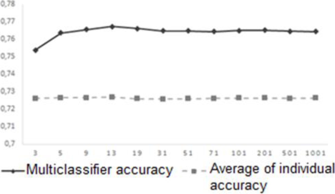
To check the behavior of SimProm, we analyze the classifier ensembles accuracy and the average of the individual accuracy. Figure 16 shows as the average of individual accuracy of the classifiers used in each classifier ensemble is much smaller than the ensemble accuracy. Therefore, the measure SimProm is the one with higher values.
Finally, we execute a correlation analysis to determine if there is a relationship among the classifier ensemble accuracy and the diversity values obtained with the new measures. Figure 17 shows the coefficient of Pearson correlation for each value of 𝑇.
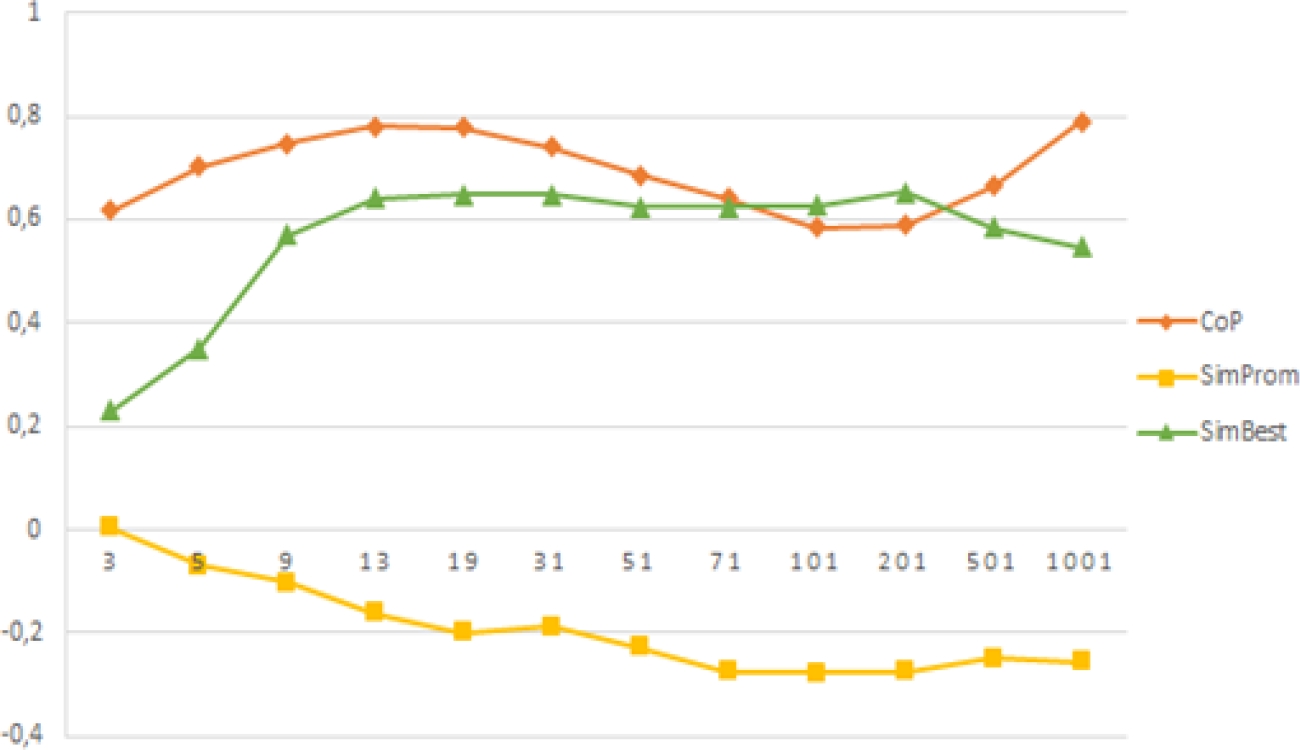
Fig. 17 Coefficient of Pearson correlation between the proposed diversity measures and the classifier ensemble accuracy
Each point represents the obtained coefficient of applying the correlation analysis of the ensembles of 𝑇 size, in the proposed measures. In this way, it is easy to study the behavior of these two elements according to the increment of the number of classifiers combined. The results show that measure based on the coverage of the classification (CoP) is the one with better correlation coefficient, moving their values between 0,6 and 0,8. Although the correlation obtained for the measure SimBest is the second better.
The coefficient is above 0,6 for most of the ensembles with 13≤𝑇≤201 size. Therefore, also we consider this measure to be positively related with the classifier ensemble accuracy.
Are interesting the results of the SimProm measure. This measure is the one with the biggest values of diversity.
However, the correlation with the ensemble accuracy is smaller than the rest and it is negative.
Therefore, high diversity values not necessarily have to be linked with the classifier ensemble accuracy. This fact is already concluded in several investigations [8, 17].
Previously, we mention that increment of 𝑇 tends to stabilize the diversity values and to form groups very well defined. Even so, the relationship with the ensemble accuracy can vary. If this relationship is demonstrated, will always be necessary an exploratory study of the results obtained in certain problem. For example, the correlation of the measures based on the similarity stay relatively stable in certain values of 𝑇 (for SimProm starting from 𝑇 = 71 and for SimBest with 13 ≤ 𝑇 ≤ 201). However, we did not observe this behavior in the CoP measure. The best correlation is with 𝑇 = 13 and starting from there it begins to decrease the correlation, until in 𝑇 = 101 increase again.
6.3 Relationship of Diversity with the Ensemble Accuracy
To complement the correlation analysis, we apply the method of the main components to determine which measures are more related with the accuracy of the formed ensemble. We calculate the measures reported in the literature on all the examples and in the Reduced Matrices (MR and MRP) to validate the previous analyzed results.
We decide to carry out the analysis of main components dividing the results of the built ensembles with 𝑇 ≤ 13, 19 ≤ 𝑇 ≤ 101 and 𝑇 ≥ 201. This is due to the behavior observed in the correlation of the proposed diversity measures with the classifier ensemble accuracy in each value of 𝑇. We make the extraction of the factors using the criterion from the auto-values superior to the unit. Also, we use the rotation varimax to facilitate the better interpret of the results.
We apply the Bartlett test in the three groups previously formed. We prove the relevance of applying the analysis of main components when obtaining a signification smaller than 0,05. For each group a total of three components are extracted and the variance described in them is around to 95% in the three intervals. Table 7 shows the extraction of each one of the variables in the three formed components for each analyzed interval of 𝑇. Also, we suppress the absolute values smallest than 0,5 to facilitate the interpretation. The line corresponding to SA represents the values for the ensemble accuracy.
Table 7 Matrix of rotated components obtained for 𝑇 ≤ 13, 19 ≤ 𝑇 ≤ 101 and 𝑇 ≥ 201
| 𝑻 ≤ 13 | 19 ≤ 𝑻 ≤ 101 | 𝑻 ≥ 201 | |||||||
| 1 | 2 | 3 | 1 | 2 | 3 | 1 | 2 | 3 | |
| SA | 0.94 | 0.88 | 0.86 | ||||||
| ρ | 0.93 | 0.901 | 0.91 | ||||||
| ρ -MR | 0.99 | 0.87 | 0.91 | ||||||
| ρ-MRP | 0.81 | 0.73 | 0.91 | ||||||
| Q | 0.96 | 0.98 | 0.98 | ||||||
| Q-MR | 0.96 | 0.95 | 0.98 | ||||||
| Q-MRP | 0.80 | 0.85 | 0.98 | ||||||
| D | 0.98 | 0.99 | 0.99 | ||||||
| D-MR | 0.99 | 0.97 | 0.99 | ||||||
| D-MRP | 0.98 | 0.98 | 0.99 | ||||||
| DF | 0.81 | 0.98 | 0.99 | ||||||
| DF-MR | 0.81 | 0.78 | 0.99 | ||||||
| DF-MRP | 0.78 | 0.50 | 0.89 | 0.99 | |||||
| R | 0.99 | 0.99 | 0.99 | ||||||
| R-MR | 0.94 | 0.97 | 0.99 | ||||||
| R-MRP | 0.99 | 0.99 | 0.99 | ||||||
| E | 0.98 | 0.96 | 0.95 | ||||||
| E-MR | 0.99 | 0.96 | 0.95 | ||||||
| E-MRP | 0.96 | 0.94 | 0.95 | ||||||
| KW | 0.77 | 0.59 | 0.88 | 0.99 | |||||
| KW-MR | 0.99 | 0.95 | 0.99 | ||||||
| KW-MRP | 0.81 | 0.55 | 0.88 | 0.99 | |||||
| k | 0.89 | 0.88 | 0.88 | ||||||
| k-MR | 0.99 | 0.81 | 0.88 | ||||||
| k-MRP | 0.72 | 0.75 | 0.55 | 0.88 | |||||
| DIF | 0.58 | 0.68 | 0.68 | 0.72 | 0.69 | 0.72 | |||
| DIF-MR | 0.88 | 0.78 | 0.69 | 0.72 | |||||
| DIF-MRP | 0.79 | 0.82 | 0.69 | 0.72 | |||||
| GD | 0.75 | 0.59 | 0.72 | 0.68 | 0.72 | 0.69 | |||
| GD-MR | 0.82 | 0.55 | 0.76 | 0.72 | 0.69 | ||||
| GD-MRP | 0.82 | 0.55 | 0.76 | 0.72 | 0.69 | ||||
| CoP | 0.59 | 0.69 | 0.63 | 0.64 | 0.71 | 0.53 | |||
| SimProm | -0.92 | -0.96 | -0.96 | ||||||
| SimBest | -0.83 | -0.55 | 0.78 | -0.57 | 0.80 | ||||
As we expected, the SimProm measure is not extracted in any moment together with the variable of the ensemble accuracy. This corroborates the results observed in Figure 17 related to the little correlation among these two variables. In the case of SimBest measure, starting from 𝑇 ≥ 19 it is included in the component that contains to the ensemble accuracy.
Therefore, we not recommend their use to build classifier ensembles with a value of 𝑇 inferior to this. On the other hand, the CoP measure is associated to the ensemble accuracy in the three groups of 𝑇, proven again their relationship with this variable.
Nevertheless, when 𝑇 ≥ 201 the expression of this measure is bigger in the first component extracted. This component does not contain the accuracy variable. In addition, we observe that DF and GD measures (independently of where they are calculated) are associated in the same component that contains the ensemble accuracy. There is a similar result with the DIF measure but the calculation over the Reduced Matrix is not related to the accuracy.
For the analysis of hierarchical conglomerates, we keep the three previous intervals. We apply the linking method among groups to form the groups with the Pearson correlation like distance. Figures 18, 19 and 20 show the result of the analysis for the three study intervals. Four groups formed according to the included measures are stood out.

Fig. 18 Dendogram formed for the diversity measures calculated on the classifiers ensembles with T ≤ 13

Fig. 19 Dendrogram formed for the diversity measures calculated on the classifiers ensembles with 19 ≤ 𝑇 ≤ 101

Fig. 20 Dendrogram formed for the diversity measures calculated on the classifiers ensembles with T ≥ 201
For 𝑇 ≤ 13, the ensemble accuracy is fundamentally associate with the measures DF, DIF and CoP, like we already observe in the analysis of main components. Interesting is the result of the two diversity measures based on the similarity of the classification (for these values of 𝑇 and for the cut point established). They form a single group that is the last one that join to the remaining ones formed in the analysis.
Starting from 𝑇 ≥ 19 the SimProm measure stays isolated of the remaining formed groups. On the other hand, SimBest begins to be related better with the ensemble accuracy. In fact, Figure 19 and Figure 20 show as how the second and fourth group respectively includes this measure together with the ensemble accuracy. Contrary to the observed with the measure CoP in the analysis of main components, except for 𝑇 ≤ 13, this measure is not included together with the ensemble accuracy in the same group.
Another important element is the association of the DF measure (independently of where it is calculated) with the classifier ensemble accuracy, as it was shown previously. Also, we observe certain relationship among the measures reported in literature calculated on the Reduced Matrix since most of them are included in the same group. Although this relationship tends to disappear when 𝑇 increasing. This proves again the previously discussed about the influence of 𝑇 values in the calculation of diversity on the Reduced Matrices.
6.4 Correlation of the Proposed Measures with the Measures in Literature
We analyze the correlation between the proposed measures with the diversity measures reported in literature. In this case, we use the artificially generated data set. Furthermore, we consider the 30,000 classifier ensembles obtained for all values of 𝑇.
We obtain the Pearson's correlation coefficient for each one of the possible combinations. In addition, we include in this study the classifier ensemble accuracy (SA) for comparison purposes. A value close to -1 indicates a negative correlation between the variables and a value close to 1 indicates a positive correlation. Otherwise, a value close to zero indicates no relation between the analyzed variables. For the analysis we use the test of correlation between paired samples (Test for correlation between Paired Samples) of the stats module of the statistical package R.
Figure 21 presents the result of the correlations between the measures. For simplicity, we only show the upper triangular matrix of the correlations. In this case, the completely white cells correspond to the cases in which the correlation is not significant. The blue color means a positive correlation and the red color means a negative correlation. The size of circle is bigger if the value is near to 1 or -1. On the other hand, the size of circle is smaller if the value is closer to zero.

We can observe that in the SimProm measure there is a positive correlation only with the SimBest measure. On the other hand, the SimBest measure also has a positive correlation with the classifier ensemble accuracy (SA). Finally, the CoP measure has a positive correlation with several measures and with the classifier ensemble accuracy.
6.5 Obtaining Classifier Ensembles in Different Scenarios
We made a last study to select classifiers ensemble in at least four different scenarios: randomly, using the first proposed measure, using the second proposed measure and using a measure from literature. In this case, we use several benchmark data sets. They are taken from the Machine Learning Repository from the University of California Irvine (MLRUCI) [50]. Table 8 shows their characteristics.
Table 8 Characteristics of the data sets
| Features | ||||
| Nro | Dataset | Instances | Nom | Num |
| 1 | Australian | 690 | 5 | 9 |
| 2 | Breast-Cancer | 683 | 9 | 0 |
| 3 | Echocardiogram | 132 | 1 | 11 |
| 4 | German_credit | 1000 | 13 | 7 |
| 5 | Heart-statlog | 270 | 0 | 13 |
| 6 | Hepatitis | 155 | 13 | 6 |
| 7 | House-votes | 435 | 16 | 0 |
| 8 | Diabetes | 768 | 0 | 8 |
| 9 | Pro-ortology | 4294 | 0 | 11 |
From each database, we take 66% of the instances for training, 17% for validation and 17% to evaluate the final classifier ensemble. The instances considered in the evaluation are not used in the training set or in the validation set. The instances considered in the validation set are not used in the training set either. On the training set, we made 33 samplings (with replacement) with a size equal to the 85% of the original size.
Each of these samples is used as training set for one of the following randomly selected learning algorithms: Logistic, KNN con k= {1, 3, 5, 7}, J48, five neural networks with different values of the learning rate and momentum (4 are randomly set and one is the default value), Random tree, DecisionStump, REPTree, NaiveBayes, ZeroR, SMO and SimpleLogistic. They are taken from the WEKA tool (Waikato Environment for Knowledge Analysis) [51].
In total, we generated a set of 33 classifiers trained with different learning algorithms and with different partitions of the original training set. After we have the classifiers trained, they are evaluated using the validation set.
Starting from the best individual classifier (best accuracy), we realize an in-depth search of classifiers that improve one of the following criteria when they are incorporated into the ensemble:
– Diversity/Accuracy using CoP,
– Diversity/Accuracy using SimBest,
– Diversity/Accuracy using the DIF literature measure.
In this study, we include the DF measure from literature because it is one of the measure that better correlation has with the ensemble accuracy according to the previous results.
We compare the obtained results with the base case of randomly selecting the classifiers to build the ensemble. We consider classifiers ensembles with size equal to nine. Once the classifier ensemble is formed, we evaluate to make the comparison in the four different scenarios.
Due to the randomness introduced when selecting the learning algorithms and the instances of each training set, we repeated the procedure 10 times and we use the average value of diversity and accuracy of the combinations found. Figures 22 and 23 show the results.


Figure 22 shows that in most of the datasets the accuracy improves when the classifiers ensembles are formed using the diversity measures. Just in two datasets (German_credit and Heart-statlog) is better the random selection to form the classifiers ensembles. Also, we observe that in several datasets the SimBest measure offer the better results.
Figure 23 shows that in most of the datasets the diversity improves when the classifiers ensembles are formed using the diversity measures. Only in a few cases of two datasets (Breast-Cancer and Pro-ortology) is better the random selection to form the classifiers ensembles. In this case, we observe again that the SimBest measure offers better results.
This study demonstrates the usefulness of the proposed measures for obtaining highly accurate or diversity classifier ensembles.
7. Conclusions
In this paper, we presented two new diversity measures based on coverage and similarity of the individual classification. In addition, we show a study of their relationship with the classifier ensemble accuracy. Besides, we analyze the diversity measures reported in literature and their behavior on a reduced dataset.
The results demonstrate how the diversity measured according to the coverage and similarity of the individual classification presents a lineal correlation with the classifier ensemble accuracy.
In case of the similarity measure, we obtained the best correlation using the output of the best individual classifier as reference point. In the case of diversity measures reported in literature, we observed a better relationship of diversity with the ensemble accuracy when the diversity is measured on a reduced data set.
This reduced data set consists in the Reduced Matrix (MR) or Positive Reduced Matrix (MRP). They are obtained starting from the output of the individual classifiers.
The DF and DIF measures show the better correlation with the ensemble accuracy. According to the results, we demonstrated that for non-pairwise measures it is better to calculate the diversity over MR or over MRP. On the other hand, for pairwise measures the best option is to continue calculating them over all the examples or depending on the measure, over MRP.
In addition, we proved that when building classifier ensembles, the number of individual classifiers influences the ensemble behavior. This influence, measured in form of diversity, means that if we increased a lot the number of classifiers the diversity can lead to a deformation of the classifier ensemble accuracy.
This deformation can be expressed in a loss of the relationship of this accuracy with the diversity. We need take into account that diversity should be controlled in the permissible limits to guarantee that the formed ensemble has the maximum behavior.
Besides, we show the correlation between the proposed measures with the diversity measures reported in literature. The most important results are: the SimBest measure has a positive correlation with the classifier ensemble accuracy (SA). On the other hand, the CoP measure has a positive correlation with several measures and with the classifier ensemble accuracy. The SimProm measure has a positive correlation only with SimBest measure.
Finally, we presented a study to select a classifiers ensemble in at least four different scenarios to demonstrate the usefulness of the proposed measures. In most of the cases, the results show that the proposed measure SimBest offers better results to form classifiers ensembles with better accuracy or diversity.
These results are compared with other three scenarios: random selection, the CoP measure and DF measure from literature.

