1 Introduction

This paper analyzes the Trajectory Tracking for a Fractional Order Nonlinear System for a Fractional Order Time-Delay Neural Network, which are forced to follow a Fractional Order Reference signal generated by a nonlinear chaotic system. The control law that guarantees trajectory tracking is obtained by using the Fractional Order Lyapunov-Krasovskii and Lur’e methodology. Chaotic behavior, as a characteristic of a dynamical system, could be desirable or undesired, depending of the current application.

In mixing substances, a chaotic behavior might improve the efficiency of the system, while in process which involves vibrations, chaos could produce critical structural failures. Consequently, it is important to be able to manipulate the chaotic nature of the system, driving a stable system to be chaotic or otherwise stabilize a chaotic system. In many applications, it is also important to change the chaotic nature of a system without losing the chaotic behavior.

Controlling and synchronizing chaotic dynamical systems has recently attracted a great deal of attention within the engineering society, in which different techniques have been proposed. For instance, linear state space feedback, Lyapunov-Krasovskii function methods [¹], adaptive control [²]. Using the inverse optimal control approach, a control law [³], which allows reproduce chaos on a Dynamical Neural Network, was discussed in [⁴]. We further extend these results to the Fractional Order Time-Delay Neural Networks case for nonlinear system trajectory tracking. The proposed new scheme is composed of a Fractional Order delayed dynamical neural identifier, which builds an on-line model for the unknown delayed neural network, and a control law, which ensures that the unknown delayed neural network tracks the reference trajectory.

There are several ways of defining the derivative and fractional integral, for example, the derivative of Grunwald-Letnikov given by eq. (1):

where [.] is a flooring-operator while the RL definition is given by eq. (2):

for (n−1<α<n) and Γ(x) is the well-known Euler’s Gamma function. Similarly, the notation used in ordinary differential equations, we will use the following notation, eq. (3), when we are referring to the fractional order differential equations where, αk∈ℝ+ which is:

The Caputo's definition can be written as:

Trajectory tracking, synchronization and control of linear and nonlinear systems are a very important problem in science and control engineering. In this paper, we extend these concepts to force the nonlinear system (Fractional Order Delayed Plant) to follow any linear and nonlinear Fractional reference signals generated by fractional order differential equations.

The applicability of the approach is illustrated by one example: chaos synchronization. In the following, we first briefly describe the dynamic of the fractional order Time-Delay Neural Network to be used.

2 Mathematical Models

The differential equation will be modeled by the neural network [⁵]:

x, u∈ℝn, A, W∈ℝnxn, where τ is the.fixed known time delay, x is the state, u is the input, A=−λI, with λ being a positive constant, W is the state-feedback matrix, and σ(∗)=tanh⁡(∗) is a Lipschitz function [⁶] such that σ(x)=0 only at x=0, with Lipschitz constant Lσ. It is clear that x=0 is an equilibrium point of this system, when u=0.

The system, to be tracked by the neural network, is defined as:

where aDtαxr, is the state, ur is the input, f(∗) and g(∗) are smooth nonlinear functions of appropriate dimensions.

As is clear, this is very general, and the model (6) can be a complex such as chaotic nonlinear system.

3 Trajectory Tracking

The objetive is to develop a control law such that the delayed neural network (5) tracks the trajectory of the dynamical system (6). We de.ne the tracking error as e=x−xr, whose derivative with respect to time is:

Substituting (5, 6, 7), we obtain:

Adding and subtracting to (8) the terms Wσ[xr(t−τ)] and α(t), we have:

where α(∗) is a function to be determined.

For system (5) to follow model (6), the following solvability assumption is needed, as discussed in [⁷]:

Assumption 1. There exist functions ρ(t) and α(t), such that:

It follows from (10 and 6) that:

So that (9) becomes:

Let us define u˜=(u−α(t)),

It is clear that e=0, is an equilibrium point of (12), when u˜=0. In this way, the tracking problem can be restated as a global asymptotic stabilization problem for the system (12).

4 Tracking Error Stabilization and Control Design

In order to establish the convergence of (12) to e = 0, which ensures the desired tracking, first, we propose the following Krasovskii [⁸] and Lur’e functional [⁹].

This is essential for the design of a globally and asymptotically stabilizing control law. We select:

The time derivative of (13), along the trajectories of (12):

We select:

Next, let consider the following inequality, proved in [¹⁰]:

which holds for all matrices X,Y∈ℝnxk and Λ∈ℝnxn with Λ=ΛT>0. Applying (17) with Λ=I to the term Ø(e,xr)TWØσT(t−τ), we get:

By simplifying (18), we obtain:

Since Ø(e,xr) is a sector function with respect to e, there exist positive constants k1 and k2 such that k1‖e‖22≤Ø(e,xr)T≤k2‖e‖22 [¹¹]. Also, since Ø(e,xr) is Lipschitz with respect to e, there exist a positive constant Lσ such that Ø(e,xr)TØ(e,xr)≤Lσ2‖e‖22. Henceforth (19) can be rewritten and then we have that:

By simplifying (20), we have:

Since Øσ is Lipschitz with Lipschitz constant Lσ [¹²], then:

Applying to:

With Lσ2 the Lipschitz constant of (23) σ(∗).

To the right hand, third term of (17), we obtain:

Now, we suggest to use the following control law:

where β is a positive constant and (R(e))−1 is a function of e: At this point, substituting (25) into (24), we obtain:

Then aDtαV(e)<0 for all e≠0. This means that the proposed control law (27) can globally and asymptotically stabilize the error system, therefore ensuring the tracking of (5) by (6).

Finally, the control action driving the recurrent neural networks is given by:

We summarize the above developed analysis in the following Theorem.

Theorem 1: The control law (27) ensures that the Time-Delay Neural Network (5) tracks the reference system (6).

5 Simulations

In order to illustrate the applicability of the discussed results, we consider we consider the following delayed neural network: aDtαxp=A(x)+Wσ[x(t−τ)]+u, where:

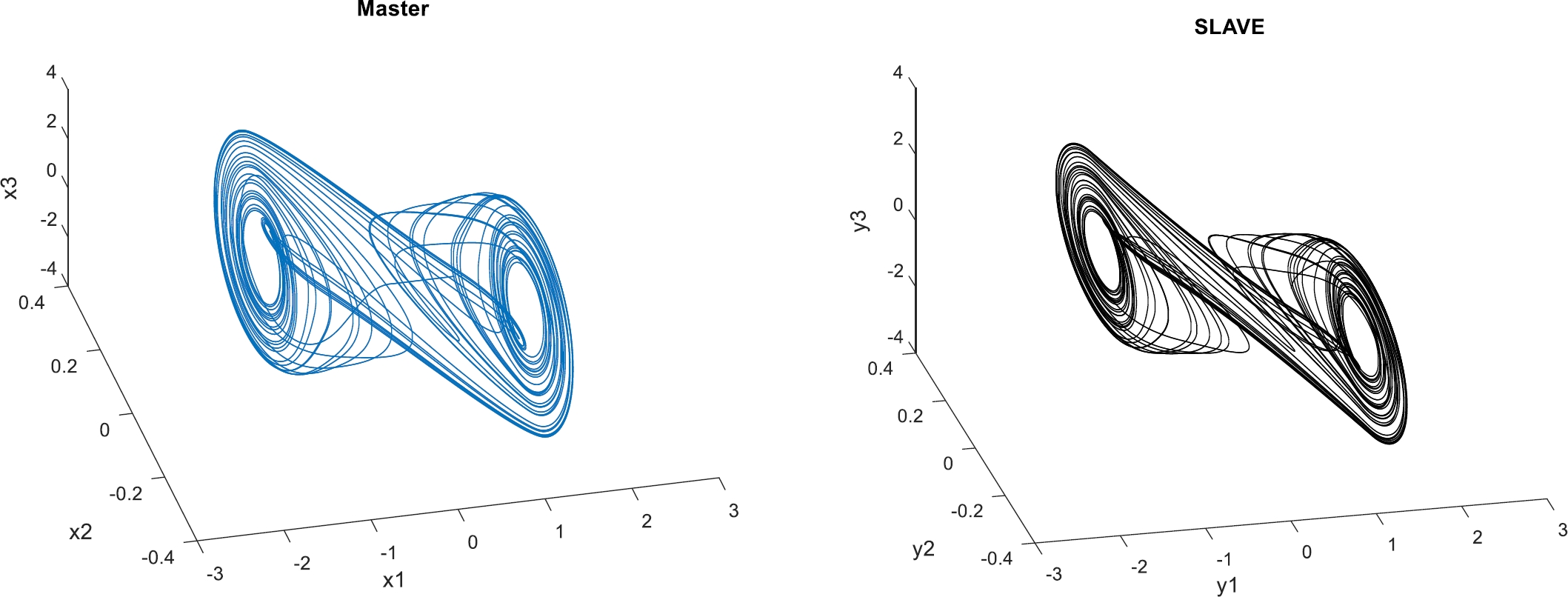
The reference model to be tracked is the Chua.s circuits [¹³]. This system is described by:

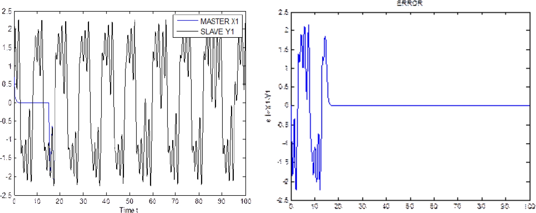
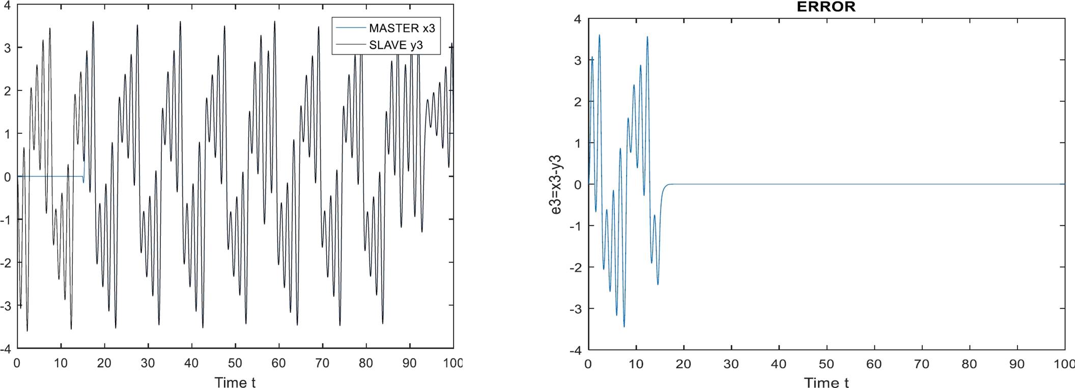
The experiment is performed as follow. Both systems, the delayed neural network and the Chua’s circuits, evolve independently until τ=15 seconds: at that time, the proposed control law (23) is incepted.

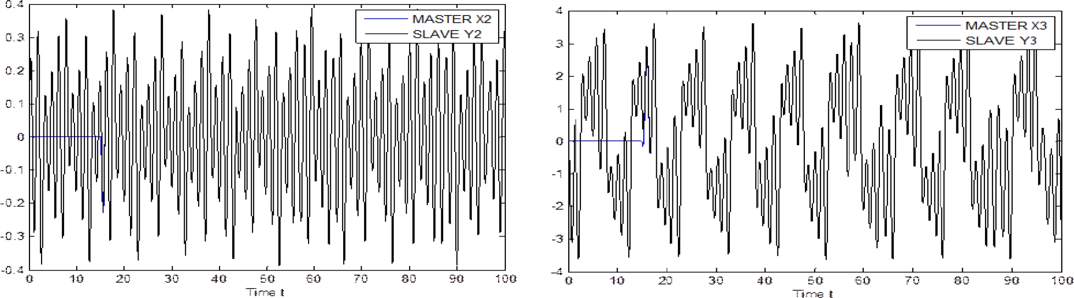
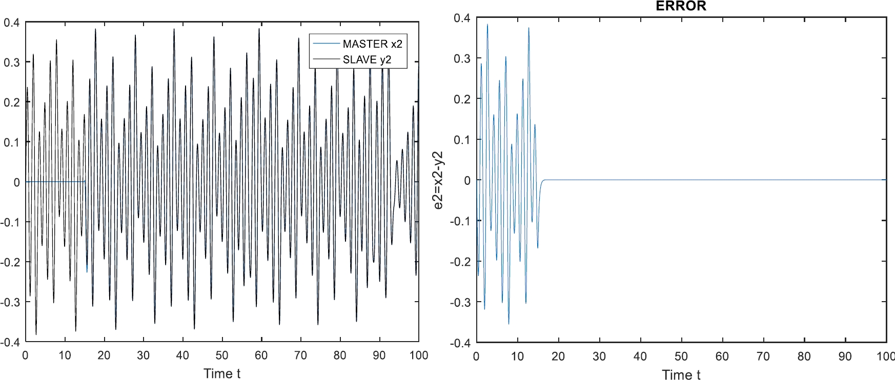
Simulation results are presented in Fig. 2, 3 y 4, for state 1, state 2 and state 3, respectively. As can be seen, tracking is successfully achieved.

Fig. 1 α=1: Simulation result for master-slave synchronization between the delayed neural network and the Chua.s circuits. The master system is coupled to the slave system with the first state variable and delay (τ=15 Sec): Three-dimensional view on the double scroll attractor generated for (a) master system and (b) slave system 

Fig. 2 Time evolution for Delayed Neural Network. Error signal (x1(t)−y1(t)) with respect to and Chua’s circuits with initial condition (0.7; 0; 0) time. 

Fig. 3 Time evolution for Delayed Neural Network. Error signal (x2(t)−y2(t)) with respect to and Chua’s circuits with initial condition (0.7; 0; 0) time 

Fig. 4 Time evolution for Delayed Neural Network. Error signal (x3(t)−y3(t)) with respect to and Chua’s circuits with initial condition (0.7; 0; 0) time 

The experiment is performed as follow. Both systems, the fractional order delayed neural network and the Chua’s circuits, evolve independently until τ=15 seconds: at that time, the proposed control law (23) is incepted. Simulation results are presented in Fig. 6, Fig. 7, Fig. 8, for state 1, state 2 and state 3, respectively. As can be seen, tracking is successfully achieved.

Fig. 5 α=0.00001: Simulation result for master-slave synchronization between the fractional order delayed neural network and the Chua’s circuits. The master system is coupled to the slave system with the first state variable and delay (τ=15 Sec): Three-dimensional view on the double scroll attractor generated for (a) master system and (b) slave system 

Fig. 6 Time evolution for the Fractional Order. Error signal (x1(t)−y1(t)) with respect to Delayed Neural Network and Chua’s circuits time, with initial condition (0.7; 0; 0) 

Fig. 7 Time evolution for the Fractional Order. Error signal (x2(t)−y2(t)) with respect to Delayed Neural Network and Chua’s circuits’ time, with initial condition (0.7; 0; 0) 

Fig. 8 Time evolution for the Fractional Order Error signal (x3(t)−y3(t)) with respect to Delayed Neural Network and Chua’s circuits time, with initial condition (0.7; 0; 0) 

6 Conclusions

We have presented the controller design for trajectory tracking determined by a Fractional Order Time-Delay dynamical network.

This framework is based on dynamic Fractional Order delayed neural networks and the methodology is based on Fractional Order Lyapunov-Krasovskii and Lur’e theory.

The proposed Inverse Optimal Control Law is applied to a dynamical fractional order delayed neural network and the Chua’s circuits, respectively, being able to also stabilize in asymptotic form the tracking error between two systems.

The results of the simulation show clearly the desired tracking. In future work, we will consider the stochastic case for the complex dynamical network.