


 nueva página del texto (beta)
 Inglés (pdf)
 Artículo en XML
 Referencias del artículo
 Enviar artículo por email
 Citado por SciELO
  Similares en
SciELO
Similares en
SciELO 
 Permalink
1 Introduction
The graph coloring problem is one of the most popular graph problems. In the decision version of the problem, the input consists of a graph and an integer
In the optimization version, the input consists only of a graph, and the goal is to find the minimum number of colors a proper coloring can have. This number is known as the chromatic number and is usually denoted by the Greek letter χ. Finding the chromatic number for arbitrary graphs is an NP-Hard problem.
Some of the graph coloring algorithms from the literature find the exact solution. However, their running time on arbitrary instances is exponential. Thus, they are useful only for small instances of the problem. For more prominent instances, the most useful algorithms are heuristics, metaheuristics, and approximation algorithms.
Most of the algorithms designed for graph coloring are heuristics, which can produce good solutions (almost near-optimal) at a reasonable computational cost [52]. Their main drawback is that they do not guarantee the solutions they produce: their quality might range from near-optimum to be arbitrarily bad. More often than not, the algorithms need to be executed repeatedly to have an idea about the given solution’s quality.
Genetic algorithms (GA) are one of these heuristics. Initially proposed by Holland in the mid-’60s, they are widely used for numerical optimization, such as prediction, scheduling, networking, speech recognition, and more [13]. However, they are regarded as poor combinatorial optimizers since they only rely on the objective function to guide the optimization process and the fact that they explore the search space by modifying bit strings. As said by Greffenstette: ”genetic operators, notably crossover, must incorporate specific domain knowledge”[28], so in order to make GA competitive when compared to other heuristics, a popular trend is to embed a local search (LS) procedure as an additional step during the execution of a standard GA. While this often produces good results, it is unclear whether the solution’s quality is due to the GA or the LS. Also, the extra computational burden of the LS procedure hinders the algorithm’s overall performance.
Another approach is to include the LS not as an additional step but within the same engine of the GA: genetic operators (selection, crossover, and mutation). This requires a careful design that considers the meaningful properties of the problem and poses an interesting tradeoff: increased performance, but at a loss of generality; since the algorithm has been designed with information on a specific problem, it will not be suitable to solve a different one.
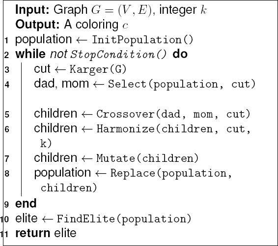
In this paper, we aim to design a GA following the latter approach. Specifically, a genetic algorithm that uses the properties of the graph coloring problem to design genetic operators through a novel methodology called structure-driven dynamic programming. We want to use the basic principles of a powerful algorithm design technique: dynamic programming to develop a genetic algorithm for graph coloring.
After designing the algorithm, we codified and tested it on a set of benchmark graph instances. Experimental results show that our algorithm is competitive with state-of-art heuristic algorithms for graph coloring. The rest of the paper is organized as follows: Section 2 presents a review of genetic algorithms used for graph coloring. Section 3 presents the proposed algorithm, with a description of the methodology used to design the genetic operators. Section 4 describe the experiments performed and show preliminary results. Finally, Section 5 presents an analysis of the experimental results, the conclusions, and possible future work directions.
2 Basic Background
2.1 The Graph Coloring Problem
Let G = (V , E) be an undirected graph. A k-coloring of the graph is a function C : V → S that assigns each vertex of the graph a label 1, 2, . . . , k ∈ S. The elements of S are called colors. A proper coloring is a k-coloring with the property that no two adjacent vértices have the same color. The chromatic number χ(G) of a graph G is the minimum k for which G has a proper k-coloring.
Most exact algorithms for the graph coloring problem are based on Dynamic Programming, Branch-and-Bound, or Integer Linear Program-ming. Among the dynamic programming algo-rithms are the O(2.4423n) algorithm of [37], the O(2.4150n) of [21], the O(2.4023n) of [10], and the O(5.283n) algorithm of [6]. These algorithms require exponential space, except for the last, which requires polynomial space. Among the Branch-and-Bound algorithms are algorithms by [8], which is based on his DSATUR algorithm, the algorithm of [9], the algorithm of [55], the algorithm of [54], and the algorithm of [23]. Among the Integer Lineal Programming algorithms are the algorithm of [45, 42, 29].
Among the heuristics for the graph coloring problem, we have the randomly ordered sequential algorithm RND [44], the maximum independent set algorithm MAXIS [7], the degree saturation algorithm DSATUR [8], and the recursive largest first algorithm RLF [38]. These algorithms run in polynomial time and do not necessarily find optimal solutions. Because of this, these algorithms are used to get an upper bound of the chromatic number.
Among the metaheuristic algorithms are pro-posals based on Simulated Annealing [33], Tabu Search [18, 31, 5, 11], Genetic Algorithms [22, 15, 25], Multiagent Fusion Search [60], Evolutionary Hybrid Algorithms [41], Local Search [32], and Ant Colony Optimization [14, 53].
2.2 Genetic Algorithms for Graph Coloring
Due to the sheer size of the search space, techniques that explore it systematically are beneficial. Specifically, genetic algorithms seem to be extremely attractive due to their (hypothetical) ability to evaluate multiple solutions at the same time, a hypothesis known as implicit paralelism. However, in practice, genetic algorithms are regarded as a poor choice for combinatorial optimization problems due mainly to the complexity of the solution to the problems themselves, which is usually not fully translated to the individuals that make up the population of the GA. For example, [16] proposed a pure GA in which solutions were codified as permutations of the vértices, which are then colored by a greedy sequential algorithm; however, the obtained results were not satisfactory since they are not able to capture the specificity of the problem [43]. As early as 1987, it has been widely accepted that, in order to solve these problems, genetic operators (notably the crossover) must incorporate in some way specific domain knowledge [28].
Most state-of-the-art proposals use local search techniques to improve the solutions generated by the genetic algorithm (either at the initialization of the population [41], at the generation of new individuals [22], or a combination of both [25]). These proposals, which combine an evolutionary base with a local search procedure, are often called hybrid algorithms. One of the first hybrid algorithms is due to [25] called HEA, which uses a greedy procedure based on the DSATUR algorithm of [8] during the initialization phase and after crossover.
More recently, [39] proposed an iterated local search algorithm based on a random walk in the search space: candidate solutions by perturbing local optimal solutions applying local search to them, and accepting them if they are within a particular acceptance criterion. They use local search as a black box that can depend on the problem to solve. [11] use a priority-based local search algorithm that introduces the concept of checkpoints, which forces the procedure to stop at specific steps and start the local search to avoid unnecessary searches.
[26] used a hybrid algorithm using a central memory that is used to produce the offspring, which in turn is further improved by a tabu search procedure and then updates back the central memory. [46] proposed a memetic algorithm combined with cellular learning automata. They further extend their proposal in [47] into a distributed Michigan GA, in which the whole population codifies a single solution, and each individual represents a single vertex that locally evolves. [3] use a repair strategy applied to children generated by a crossover to find university timetables. [61] solve a similar scheduling problem of assigning tasks to teams of agents by using modified genetic operators with shuffled lists and chaotic sequences.
2.3 Genetic Operators Designed for Combinatorial Optimization
Genetic algorithms have also been applied to different combinatorial optimization problems, other than graph coloring, with varying degrees of success. For example, [56] propose a genetic algorithm for the traveling salesman problem (TSP), which is another well known NP-Hard problem [35]. In TSP, a list of n cities is given, with different costs of moving from one city to another, and the goal is to find a route that visits all cities exactly once while minimizing the total cost (some variants also require that the tour finishes on the starting point).
In their proposal, Thanh et al. use three different types of crossover: MSCX (Modified Sequence Constructive Crossover), which construct new individuals by sequentially selecting the next ’legitimate’ gene for either parent, that is, the next city that appears on tour in one of the parents that is not yet visited, and that posses the minimum cost. This crossover operator is further expanded to the MSCX radius variant, in which the next r ’legitimate’ genes are selected instead of just 1 (r being a parameter of the procedure). The main idea behind these operators is to select edges with small values that are preserved within tours, thus maintaining the parents’ sequence of cities. A third crossover, called RX, is used when the population’s diversity falls below a given threshold, randomly selecting genes from one parent and filling the remaining positions with genes from the other
Multiple TSP is a variant of the original TSP in which there are m > 1 salesmen that must visit n cities, with m < n. [12] proposed a two-part chromosome representation, in which each individual is composed of two different parts: the first n genes being a permutation of the n cities to visit, and the second part being a vector of m integers (x1, ..., xm) satisfying x1 + ... + xm = n where xi > 0, i = 1, ..., m. This vector indicates how many cities are visited by each of the m salesmen. New individuals are generated via a variation of classic ordered crossover [27] used on the chromosome’s first section: a random sequence of genes is copied from one of the parents, the remaining positions are filled with the genes of the other in the order in which they appear. The second part of the chromosome only is permuted from the first parent to maintain a valid vector with the properties specified before.
[62] improved the two-part chromosome crossover by using the second part’s information to better select genes on the first. ’Sub-routes’ are randomly selected from one parent for each salesman, with the remaining cities are also randomly assigned, following their order on the second parent. This way, the building blocks that make up good routes are preserved while also maintaining a greater diversity of the population since it is possible for children to have routes of different sizes that were not present on their parents.
3 Structure-Driven Dynamic Programming for Graph Coloring
In this paper, we present a new type of genetic algorithm designed explicitly for combinatorial optimization, called Structure-driven Dynamic Programming for Graph Coloring (SDP-GC). The proposed algorithm was designed to incorporate the dynamic programming methodology’s main principles into the genetic algorithms paradigm. The proposed algorithm explores the solution space following using a relaxed version of the structured way in which dynamic programming exploits structural properties of the problem to build solutions to larger subproblems by combining solutions of smaller subproblems. These ideas are implemented by incorporating the dynamic programming principles into the genetic operators to take advantage of the graph coloring problem’s particular structural properties.
3.1 Overview
Unlike many previous proposals [63, 19, 26] that rely on having an excellent first generation, SDP-GC creates its initial population by assigning a color uniformly at random to every node in the input graph G = (V , E).
Then, for each generation, SDP-GC partitions G = (V , E) into two subgraphs to define two sub-problems that can be colored with more ease. When selecting these partitions, SDP-GC balances the dynamic programming principle of having weakly interacting sub-problems with the genetic algorithms’ strategy that uses population diversity as a way to explore the solution space. More specifically, SDP-GC uses Karger’s algorithm [34] (also known as the randomized min-cut algorithm) to look for partitions with small cut-sets in a randomized fashion.
Please note that SDP-GC can be extended to work with partitions of more than two components.
The first step to designing a dynamic program-ming algorithm is to define what is considered a ”subproblem.” One option, naturally, is to partition the given graph G = (V , E) into subgraphs, which due to being smaller than the original graph they can be colored with more ease. There are virtually endless ways to partition a graph into subgraphs: however, for our purposes, we must take into account an important detail: one could think that, once these subgraphs are properly colored, then a coloring for the original graph can be created just by joining them back, but this is not necessarily true. We must consider the set of all edges that have one endpoint in a subset and the other endpoint in a different subset (called a cut-set): these edges can (and often will) result in conflicts due to their endpoints being assigned the same color in their respective subgraphs.
In the next step, SDP-GC selects individuals based on the fitness of their partitions. This way, individuals with a global bad fitness but with reasonable solutions in either partition will have a better chance of passing that sub-solution to the next generation. The rationale behind selecting individuals is to mimic how dynamic programming algorithms build their solutions from solutions to smaller sub-problems.
The crossover operation creates new individuals (colorings) as the union of the colorings of selected partitions. Then, SDP-GC uses procedure Harmonize to look for the permutation of colors assigned to nodes of one of the partitions that minimize the number of monochromatic edges in the cut-set. This procedure is essential because the two partitions’ colorings were independently computed (See Figure 1).
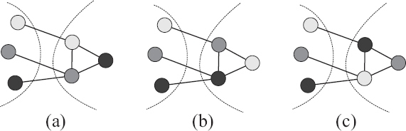
Fig. 1 An example of harmonization between colorings of two subgraphs. Figure (a) shows the original sub-solutions, as computed independently on each subgraph by the algorithm; this coloring has two conflicts on the cut-set. Figure (b) shows the colors of the right subset permuted, which reduces in 1 the number of conflicts. Figure (c) shows a different permuting, which effectively eliminates all conflicts that arose when the sub-solutions were joined. Note that, even when the colors of the right subset were changed, the solution remains essentially the same
Lastly, SDP-GC uses traditional mutation and replacement procedures to complete the construction of the next generation of individuals.
The following subsections present detailed information about each step of the algorithm, explaining the ideas used to implement the intuition presented in this subsection, but before we will introduce some notation. Let G = (V , E) be an undirected graph.
Then for any subset of vértices X ⊆ V , the sub-graph induced by X is denoted by H = (X, se(X)), with se(X) being the subset of E that contains only the edges whose both endpoints belong to X:
Definition 1. For a graph G = (V , E) and a subset of nodes X ⊆ V :
Similarly, for any subset of vértices X ⊂ V , we represent by ct(X) as the cut-set, that is, the subset of E that has one endpoint in X and the other endpoint in a different subset of vértices.
Definition 2. For a graph G = (V , E) and a subset of nodes X ⊂ V :
Given a vertex v ∈ V , we denote by N(v) the neighborhood of v, that is, all other vértices u ∈ V that share an edge with v.
Definition 3.
Lastly, we will say that an individual is represented by a coloring c, which is defined as a function c : V → {1, 2, ..., k} where k is the maximum number of available colors.
3.2 Initialization
As stated in the previous section, the algorithm’s initialization is done via an efficient random initialization. This procedure takes two integers: the population size p and the maximum number of colors admitted k and creates the initial population as a matrix of p × |V| by merely assigning a color uniformly at random from [0, k) to each gene. It is important to note that given the random nature of this approach, invalid colorings may be produced.
3.3 Partitioning the Graph
At each generation the graph is partitioned into different subgraphs to maintain diversity in the population and explore new solutions using Karger’s algorithm, which is entirely based on a simple operation called edge contraction. To contract an edge e = (u, v), we merge the two vértices u and v into one ’super-vertex’ uv, eliminate all edges connecting u and v while retaining all other edges in the graph.
This new graph may contain parallel edges but no self-loops. The algorithm consists of |V| − 2 iterations; at each of them, an edge is picked uniformly at random to be contracted. Since each iteration reduces the number of vértices in the graph by one, after |V| − 2 iterations, the graph consists only of two vértices. The general outline of this procedure is presented on Algorithm 2.
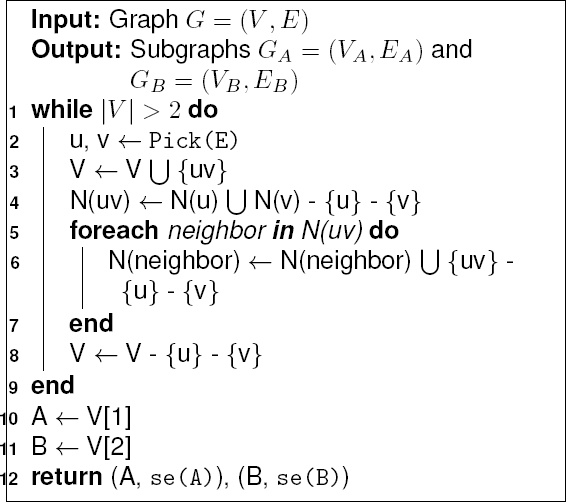
In the Karger’s algorithm, procedure Pick(E) choses a random edge e = (u, v) ∈ E, and procedure se(X) returns the subset of edges whose both endpoints are elements of the given set X, just as stated on Definition 1.
The original algorithm has a probability of
3.4 Selection
In order to maintain simplicity, the selection technique used is the classical roulette wheel selection proposed by DeJong[17], which is slightly inefficient (its original complexity is O(n2)), but it is simple and easy to implement.
Being a fitness-proportional selection technique, it is necessary to define the fitness function before proceeding any further. The fitness function we use is simply the percentage of a subgraph induced by A ⊆ V that is colored appropriately, ignoring all edges in the other subgraph and on the cut-set. Using this approach, individuals have more than one fitness value.
Definition 4. For an individual i and a subset of vértices A ⊆ V , their fitness is:
In Equation (1), 1predicate denotes the random variable that takes the value 1 if predicate is true, and 0 otherwise. Note that using this fitness function, values are restricted to the interval [0, 1].
The selection method Select is essentially the classical roulette wheel, with the difference that the first parent is selected based on their fitness in subgraph GA = (A, se(A)). The second parent is selected based on their fitness in subgraph GB = (B, se(B)). This procedure is outlined in Algorithm 3.
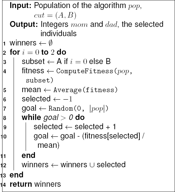
In the Select, procedure ComputeFitness applies Equation 1 to each individual of the population using the given subset and returns a vector of |pop| elements, which are the fitness values of the population on the subgraph induced by the subset. Procedure Average takes this vector and computes the arithmetic mean. Finally, procedure Random(A, B) returns a real number taken uniformly at random from the interval [A, B]. As a return value, Select returns a 2-value vector, which are the indexes of the selected individuals.
3.5 Crossover
With the two individuals that best color the subgraphs selected, we need to combine them to produce the new individuals. This is very simple and can be seen as a variant of the uniform crossover, initially proposed by [2].
Given a cut x = (A, B) and two parents mom and dad, each crossover operation produces two new individuals: the first contains the colors of the nodes in subset A from mom and the colors of the nodes in subset B from dad. The second individual is generated in the same way, but with the parents reversed. This procedure is outlined in Algorithm 4.
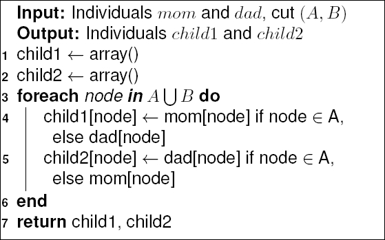
As stated at the start of this section, the main issue with this approach is that good coloring of the subgraphs might not result in a good coloring of the whole graph when combined since edges on the cut-set might create conflicts when the sub-solutions are put back together. To reduce the likelihood of conflicts, we designed a special procedure to define a mapping coloring function that can reduce the number of conflicts when re-joining sub-solutions.
This can be done in the following way: given a graph G = (V , E), a coloring c and a cut x = (A, B) we create a complete 2k bipartite weighted graph Hk,k = (W , F), representing ’bags’ (or clusters) of nodes. The first k bags represent the colors used on the sub-solution induced by subset A, and the other k bags represent the colors used on the sub-solution induced by subset B. Initially, all edges f ∈ F weight zero, and then, the cut-set of the original graph is used to modify these weights: for each e = (u, v) ∈ ct(A) we proceed to increase the weight of the edge f = (c(u), c(v)) ∈ F by one: this represents that if the labels assigned to u and v were the same on their respective sub-colorings, one conflict would arise in the complete solution when they are put back together. If c(u)! = c(v), then the weight of the edge f′ = (c(v), c(u)) is increased by 1 as well.
With edges on the cut-set analyzed, the next step consists of creating a perfect matching between A and B: each of the k bags of A must be joined with exactly one bag of B. To achieve this, we proceed to prune the graph H by repeatedly deleting the edges with the largest weight, until the perfect matching is done. Given the case that all edges of the resulting perfect matching weight zero, we have found a mapping coloring function that, virtually, eliminates all conflicts on the cut-set.
A few polynomial-time algorithms are designed to find minimum-weight perfect matchings (a fundamental combinatorial optimization problem known as the assignment problem).
We decided to use the Hungarian algorithm due to its simplicity. The details of this algorithm are beyond the scope of the present work. However, since assignment is a common problem, it has been implemented as a library and is available in many programming languages. The complete procedure is outlined in Algorithm 5.
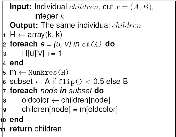
In procedure Harmonize, Munkres is an imple-mentation of the Hungarian algorithm that takes a k × k weight matrix and returns a function m that takes a color oldcolor and returns a newcolor. It is named so due to one of the people who helped develop the algorithm, James Munkres [50].
3.6 Mutation
In our original proposal, we use a simple Gaussian or ’flip’ mutation: each gene of the individual is considered independently: for each of them, a biased coin is flipped, with probability PM = 1/|L| of landing heads: if so, the gene is replaced with another color in [0, k) taken uniformly at random; otherwise, the gene is left unchanged.
3.7 Replacement
The last step of an iteration of the algorithm is the replacement, which follows a simple rule: the best of the two children generated by crossover replaces the worst of the two parents, even if it has a lesser fitness itself.
This is done to maintain the population’s genetic diversity since new, exploratory solutions that might not be as good at the moment are allowed to survive on the population. If the two parents have the same fitness, then either is selected at random to be replaced. Given that the best of the two parents is never replaced, our proposed GA has elitism.
3.8 Analysis
3.8.1 Properties
Now let us discuss some of the properties of our proposal. First, we will argue that the harmonization procedure effectively reduces con-flicts when re-joining sub-solutions back together. Once the Hungarian algorithm has found a perfect matching, the next step is to apply the mapping coloring function defined by it to one of the two subsets. Which one of the subsets is decided randomly based on subset’ size: smaller subsets have an increased chance of being modified than larger ones.
As we stated before, by mapping colors, solutions remain, in essence, the same since the labels (colors) of the clusters are modified, but the nodes that make up the clusters remain the same. However, this change reduces conflicts on the cut-set. Though it may seem obvious, it is worthwhile to take a closer look at this observation. First, it is useful to define a function to compute the number of conflicts that a coloring produces on a graph.
Definition 5. Let G = (V , E) a graph, and c a coloring of G. Then, for any subset A ⊆ V , the number of conflicts that c induces on A is:
Lemma 3.1. Let G = (V , E) a graph, x = (A, B) a cut of G, c(X) a coloring of a subset X ⊆ V and c′ a mapping coloring function of c obtained through the Hungarian method described above. Then:
Proof. The proof is by contradiction. First, note that mapping coloring functions never creates more conflicts on their subsets since the labels of colors are only ’rotated,’ and thus, the number of conflicts within the subset remains the same. Next, note that mapping coloring functions neither increases the number of conflicts with vértices of other subsets that do not belong to the cut-set since they do not interact with each other. Based on these two observations, we only need to prove that the number of conflicts on the cut-set never increases with mapping coloring functions.
Recall that the graph Hk,k used to find the mapping coloring function is created using the number of possible conflicts between all the k labels used on the coloring. By applying the Hungarian algorithm on H, we effectively found a perfect matching of minimum cost, or, in our context, a mapping coloring function of minimum conflicts. Proof for the Hungarian algorithm is beyond the scope of this work but can be checked in [36], among other sources.
Now we would like to emphasize the Karger algorithm. Through our experimental results, we discovered that more times than not, if the Karger algorithm was executed a proper amount of times to guarantee a minimum size cut to be found, the GA made little to no progress, and the reason is straightforward. Most times, the cut found was essentially the same.
If the algorithm is let to run with the same cut every generation, it is not exploring the search space thoroughly, and it gets stuck on local optima with ease. Not only that but the extra computational burden of repeating Karger’s algorithm a large number of times at each generation also hinders the proposal’s overall performance. With these two facts in mind, executing Karger’s algorithm to obtain a genuinely random cut results in increased performance and helps to balance the exploration-exploitation tradeoff, which is a common issue for most evolutionary algorithms.
3.8.2 Complexity
To establish our algorithm’s computational com-plexity, let us examine the complexity of each of the steps that make up a single generation step. Let G = (V , E) be an arbitrary graph, and let n = |V| and m = |E|. Then:
— Procedure Karger: The algorithm is executed by contracting the edges of E until only two nodes remain. The best implementations are known to have a O(m) running time. [34]
— Procedure Select: The complexity of the procedure depends on the selection method used. Since classical roulette wheel is used, in this case, its complexity is O(n2). [13]
— Procedure Crossover: The crossover is executed by copying the colors from parents to offspring, which is made in linear time O(n).
— Procedure Harmonize: The Hungarian algorithm is executed over a (k × k) matrix, being k the current maximum allowed number of colors to use. It can be implemented to run in O(k3), and, given the fact that k < n (since a n-coloring is trivial), then its complexity is O(n3). The remaining part of the algorithm is to map the colors made once for each node, and thus linear in time O(n).
— Procedure Mutate: Mutation is made over each node, so it is linear in time O(n)
— Procedure Replace: Replacement is just the copying of one individual into another, and so is linear in time O(n)
So with these information, the complexity of a single step generation of the proposal is O(n3).
4 Experimental Results
This section presents the results obtained through a series of experiments that show that the SDP-GC algorithm is a feasible alternative to state-of-the-art algorithms, producing competitive results for the quality of the solutions and running times. The algorithms and data structures described in the previous chapter were coded in Python 3.7.2, using NumPy 1.16.2.
The graphs used as input are a subset of the DIMACS benchmark graphs for the graph coloring problem, which is available to consult in the following link: http://mat.gsia.cmu.edu/COLOR/instances.html.
The present section is organized as follows: section 4.1 presents the experiments that were conducted during the initial phase of the SDP-GC algorithm and is intended to explain some of the design decisions. Next, Section 4.2 compares the performance of SDP-GC in a broader set of benchmark instances against the result of some of the best state-of-art algorithms found in the literature.
4.1 Design Decisions
This phase’s main objective is to explain some of the decisions that were made during the development of the SDP-GC algorithm. As presented in the previous section, the critical operation that guides the algorithm is the Karger procedure that generates random cuts. Although it might seem at first glance that working with minimum cuts is better, the initial results of the algorithm were discouraging. After analyzing the algorithm’s output, we made an interesting observation: in most graphs, the minimum cut is an isolated vertex.
This provokes that the algorithm behaves in an undesired way since colorings on isolated vértices cannot be further improved or modified. This observation led to the hypothesis that it might be better for the algorithm to work with trully random cuts, even if they are not minimum. Hence, the first set of experiments were designed in order to compare the variant of the algorithm that generates its cuts with only one Karger iteration (named 1Karger) and the version of the algorithm that works with the recommended number of Karger iterations described in [48] (named FullKarger).
The next observation done was made during the curse of the previous experiments: sometimes, the algorithm failed to declare a valid coloring, even when tremendous progress had been made. It is worth to mention that, at this moment in the history of the algorithm, a different fitness function was being used: the fitness of an individual was simply the number of edges that were conflict-free. While this fitness function fulfilled its purpose (better solutions had higher values), it was not giving a clear idea of how much work was left to do. It is for this reason that we introduced the new fitness function given in Definition 4. With this new fitness function, experiments showed that elite individuals were close to a correct solution when a run was declared unsuccessful.
For this reason, we introduced the notion of
The notion of the
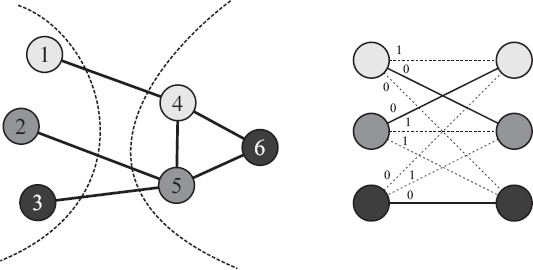
Fig. 2 An example of the harmonization procedure. Sub-solutions of the graph use three colors: white, gray, and black. The complete bipartite weighted graph of the right represents all the possible interactions between these colors. Weights on the (white, white), (grey, grey), (grey, black), and (black, grey) edges were increased to indicate potential conflicts. The continuous lines are the minimum-weight perfect matching between both sides that eliminates all the conflicts

Fig. 3 Performance comparison of 1Karger to FullKarger. The top row shows on the x-axis the name of the graph instances and on the y-axis time needed to complete. It is clear that the increase in the number of iterations of the Karger procedure also dramatically increases the running time. The bottom row shows on the x-axis the names of the same graph instances of the top row, and on the Y-axis the number of iterations needed to find the χ(G): on most graphs, 1Karger cuts almost by half the number of iterations. Boxes represent the values between the 9th and 91st percentile
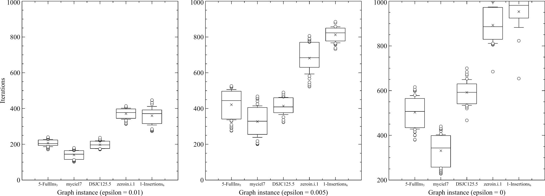
Fig. 4 Performance comparison of 1Karger version of the algorithm with varying values of . On the y-axis is the name of the graph instances used, and on the x-axis, the required number of iterations to find a correct solution. As expected, the greater the value of
The third and final observation that determined the algorithm’s design was made during the previous two experiments. When monitoring the algorithm’s execution state, we noticed that progress towards a valid coloring is made much more rapidly in the early stages of the execution than in the final stages. It would not be uncommon that, once a specific fitness is reached, the algorithm would go for a relatively large number of ”dead” iterations, in which no progress is made. After analyzing the outputs of some executions, we discovered the reason behind this behavior: most of the progress the algorithm makes is made during the harmonization procedure: is in this stage where the number of conflicts presents the most significant decrease.
Thus, once the graph has few conflicting edges, it is hard to reduce its numbers if those edges are not in the cutset.
To avoid this problem, we slightly modified the Karger procedure with the notion of strict cut. Typically, cuts are created entirely at random, allowing the algorithm to explore the search space freely. However, once the elite individual fitness value surpasses a defined threshold, cuts start to be created strictly: this means that, instead of selecting the first edge to start the cut uniformly at random, in a strict cut, we deterministically select a conflicting edge to begin the creation of the cut. This simple rule assures that at least one conflicting edge will be inside the cut-set, and thus, the algorithm will be able to eliminate said conflict.
4.2 Performance Comparison
For this section, a subset of 46 benchmark graphs commonly used on the literature was selected to conduct the experiments. The algorithm was executed a set amount of times for each one, and the best result obtained is reported. These results are compared against those collected from a survey made on heuristic algorithms for graph coloring. The algorithms reviewed are listed as follows:
— HEA (Galinier and Hao, 1999) [25],
— CRI (Herrmann and Hertz, 2000) [30],
— CHECKCOL (Caramia et. al., 2006) [11],
— MMT (Malaguti, Monaci and Toth, 2008) [41],
— IPM (Dukanovic and Rendl, 2008) [20],
— AMACOL (Galinier, Hertz and Zufferey, 2008) [26],
— FOO-PARTIALCOL (Blochliger and Zufferey, 2008) [5],
— MACOL (Lu and Hao, 2010) [40],
— Evo-Div (Porumbel and Kuntz, 2010) [51],
— QA-col (Titiloye and Crispin, 2011) [57],
— EXTRACOL (Wu and Hao, 2012) [58],
— EXSCOL (Wu and Hao, 2012) [59],
— PASS (San Segundo, 2012) [54],
— HPGA (Abbasian and Mouhoub, 2013) [1],
— B&C (Bahiense and Ribeiro, 2014) [4],
— RLS (Zhou, Hao and Duval, 2016) [64],
— SDGC (Galan, 2017) [24],
— HEAD (Moalic and Gondran, 2018) [49].
Figure 5 shows the overall algorithm’s performance. On the universe of graphs selected, in half of them (23 instances) our proposal was able to find colorings using the same amount of colors reported on the literature as being the optimal. On the other half, in 11 instances (23%) the colorings found by our algorithm fall behind the results reported in the literature by 1 color. These instances (as well as some results from other authors) are reported in Table 2.
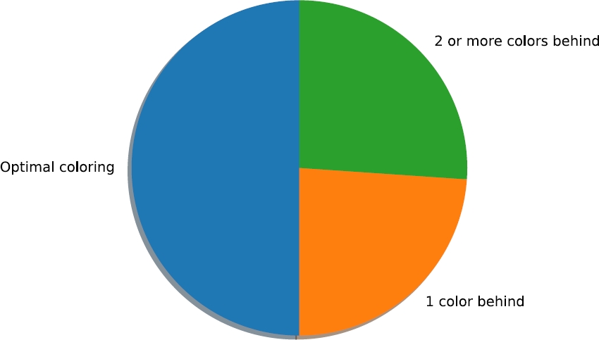
Fig. 5 Overall performance of SDP-GC against the reviewed algorithms. On half of the instances (23) SDP-GC was able to find the optimal coloring, whilst in almost a quart (11) the best coloring found is only 1 color behind the best colorings reported. In the remaining graphs, the coloring founds use 2 or more colors than the best colorings reported
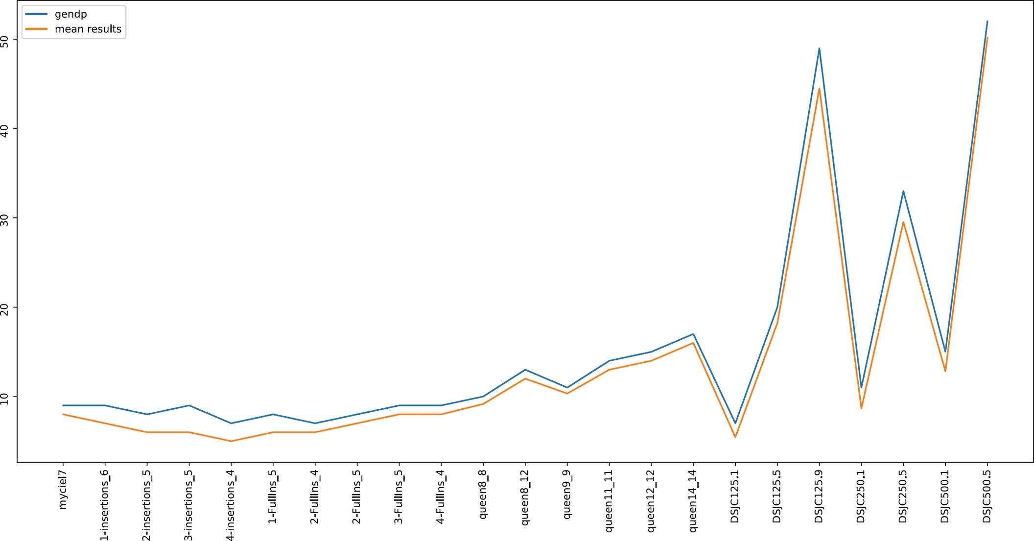
Fig. 6 Performance comparison of SDP-GC against the mean results found in the literature in unfavorable instances. When compared with a broad amount of proposals, the performance of SDP-GC is quite close to the mean performance
Table 1 Instances in which SDP-GC found the optimal coloring reported in the literature
| Instance | SDP | Instance | SDP |
| myciel3 | 4 | myciel4 | 5 |
| myciel5 | 6 | myciel6 | 7 |
| 1-Insertions_4 | 5 | 1-Insertions_5 | 6 |
| 2-Insertions_3 | 4 | 2-Insertions_4 | 5 |
| 3-Insertions_3 | 4 | 3-Insertions_4 | 5 |
| 4-Insertions_3 | 4 | 1-FullIns_3 | 4 |
| 1-FullIns_4 | 5 | 2-FullIns_3 | 5 |
| 3-FullIns_3 | 6 | 3-FullIns_4 | 7 |
| 4-FullIns_3 | 7 | 5-FullIns_3 | 8 |
| queen5_5 | 5 | queen6_6 | 7 |
| queen7_7 | 7 | queen10_10 | 12 |
| queen13_13 | 15 |
Table 2 Instances in which SDP-GC failed to find optimal colorings by 1 color. Empty cells means that the corresponding instance was not reported by the algorithm’s authors
| Instance | Best k | SDP-GC | PASS | IPM | Evo-Div | SDGC |
| myciel7 | 8 | 9 | 8 | 8 | ||
| 2-FullIns_4 | 6 | 7 | 6 | 6 | ||
| 2-FullIns_5 | 7 | 8 | 7 | |||
| 3-FullIns_5 | 8 | 9 | 8 | |||
| 4-FullIns_4 | 8 | 9 | 8 | |||
| queen8_8 | 9 | 10 | 9 | |||
| queen8_12 | 12 | 13 | 12 | 12 | ||
| queen9_9 | 10 | 11 | 10 | 10 | 11 | |
| queen11_11 | 13 | 14 | 13 | 13 | 13 | |
| queen12_12 | 14 | 15 | 14 | 14 | 14 | |
| queen14_14 | 16 | 17 | 16 | 16 |
Table 3 shows the results on instances in which the colorings found by SDP fall behind the best ones reported in the literature by 2 or more colors. It is important to note that, even when SDP-GC wasn’t able to replicate the best results, it produced colorings using the same amount of colors (or even less) than others authors.
Table 3 Instances in which SDP-GC failed to find optimal colorings by 2 or more colors. Empty cells means that the corresponding instance was not reported by the algorithm’s authors
| Instance | Best K | SDP-GC | IPM | PASS | EXSCOL | MMT |
| 1-Insertions_6 | 7 | 9 | 7 | 7 | ||
| 2-Insertions_5 | 6 | 8 | 6 | |||
| 3-Insertions_5 | 6 | 9 | 6 | |||
| 4-Insertions_4 | 5 | 7 | 5 | 5 | ||
| 1-FullIns_5 | 6 | 8 | 6 | 6 | ||
| DSJC125.1 | 5 | 7 | 6 | 5 | 7 | 5 |
| DSJC125.5 | 17 | 20 | 19 | 19 | 20 | 17 |
| DSJC125.9 | 44 | 49 | 46 | 44 | 44 | |
| DSJC250.1 | 8 | 11 | 10 | 9 | 10 | 8 |
| DSJC250.5 | 28 | 33 | 34 | 31 | 28 | |
| DSJC500.1 | 12 | 15 | 14 | 14 | 12 | |
| DSJC500.5 | 47 | 52 | 62 | 51 | 48 |
When compared with those reported, experimental results show that SDP-GC produces competitive results in most instances, while in others, the colorings found are close enough to be acceptable.
5 Conclusions and Future Work
The proposed algorithm was built using a standard, feature-less genetic algorithm, which is often regarded as a poor choice to solve combinatorial optimization problems. Through a careful design of genetic operators that incorporate information inherent to the graph coloring problem’s structure, and using principles inspired by dynamic program-ming, a fast and straightforward genetic algorithm was designed.
The proposed algorithm was codified, and a series of experiments were carried out over a set of benchmark instances to analyze its performance. Although the results were initially not as good as expected, these results helped to make some decisions during the initial stages of development. In the end, they lead to the final design of the genetic operators that allowed the proposed algorithm to improve its performance, which makes it a competitive and interesting alternative for graph coloring.
Although dynamic programming principles were successfully applied to a genetic algorithm for the graph coloring problem, a generalization of it to be applied to a broader amount of problems would also be of interest. This is the main topic of research in which the authors are interested at this moment.

