SciELO - Scientific Electronic Library Online

 
vol.25 número1Lexical Patterns Based on Maximal Frequent Secuences for Automatic Keyphrase ExtractionDiscretization Accuracy of Continuous Signal Peak Values in Limited Bandwidth Systems índice de autoresíndice de materiabúsqueda de artículos
Home Pagelista alfabética de revistas  

Servicios Personalizados

Revista

Articulo

Indicadores

Links relacionados

  • No hay artículos similaresSimilares en SciELO

Compartir


Computación y Sistemas

versión On-line ISSN 2007-9737versión impresa ISSN 1405-5546

Comp. y Sist. vol.25 no.1 Ciudad de México ene./mar. 2021  Epub 13-Sep-2021

https://doi.org/10.13053/cys-25-1-3888 

Articles

Analog Algorithms with Discontinuous States and Non-Unique Evolution Operators: Computability and Stability

Zvi Retchkiman Konigsberg1  * 

1Instituto Politécnico Nacional, Centro de Investigación en Computación, Mexico


Abstract:

In this work computability and stability issues for analog algorithms with discontinuous states and non-unique evolution operators are studied. The notions of analog algorithm and dynamical system are postulated to be equivalent. The stability and stabilization concepts for analog algorithms are defined. The stability and stabilization presentation starts concentrating in continuous and discrete dynamical systems i.e., analog algorithms, defined by differential or difference equations, and continues considering Lyapunov energy functions for analog algorithms with continuous and discontinuous states. Dynamical systems with non-unique evolution operators are also studied.

Keywords: Analog algorithms; dynamical systems; discontinuous; non-unique evolution operators; stability; Lyapunov functions

1 Introduction

This work presents analog algorithms with discontinuous states and non-unique evolution operators. Bournez, Dershowitz and Neron [1] have formalized a generic notion of analog algorithm. They provide postulates defining analog algorithms in the spirit of those given for discrete algorithms [2], and continue proving some completeness results. The notions of analog algorithm and dynamical system are postulated to be equivalent.

Retchkiman and Dershowitz [3] have studied the stability and stabilization concepts for analog algorithms. They first considered the stability and stabilization issues concentrating in continuous and discrete dynamical systems i.e., analog algorithms described by differential or difference equations. This paper extends these results considering Lyapunov energy functions for analog algorithms with continuous and discontinuous states which applies to many classes of dynamical systems including hybrid systems and switched systems. Dynamical systems with non-unique evolution operators are also presented.

The paper is organized as follows. In section 2, the paper written by Retchkiman and Dershowiz related to analog algorithms is first reviewed. The stability and stabilization concepts for analog algorithms are defined. Section 3 presents an application example. Section 4 discusses the stability concept for analog algorithms with continuous and discontinuous states in terms of Lyapunov energy functions, and finally section 5 discusses analog algorithms for dynamical systems with non-unique evolution operators.

2 Analog Algorithms, the Church-Turing, Stable Algorithms and Stabilization of Unstable Analog Algorithms

In this section, the work presented in [3] and the references therein is recalled.

Definition 1. A dynamical system is a four-tuple {T,X,A,ϕϕt}, where T is called the time set, X is a state space (a metric space with metric d), A is the set of initial states A⊂⊂X and ϕϕt:X→→X is a family of evolution operators parameterized by t∈∈T satisfying the following properties: for x∈∈X, ϕϕ0(x)=x, and ϕϕt+s=ϕϕt∘∘ϕϕs.

Remark 2. Note that in our definition of dynamical system, it is allowed to have, in general, more than one evolution operator.

Dynamical systems are classified based on the properties of T, X and ϕϕt. The time set T is it continuous or discrete?. The state space X is it finite or infinite?, is it continuous or discrete?. Is it X finite-dimensional or infinite-dimensional?. The map ϕϕt: Deterministic or stochastic?, autonomous or time-dependent?, invertible or not?, etc. Some examples are: Turing machines, finite state automata, continuous systems, discrete systems, discrete event systems and hybrid systems (to mention some).

When T=ℛℛ=(−−∞∞,∞∞), we speak of a continuous-time dynamical system, and when T=N={0,1,2,⋯⋯} we speak of a discrete-time dynamical system. We will consider T equipped with the absolute value as a normed space i.e., (T,|⋅⋅|).

A dynamical system is generally defined by one or more differential or difference equations There are other important classes of dynamical systems as those defined by continuous differential equations, functional differential equations, semi-groups, to mention some.

Remark 3. When dealing with continuous dynamical systems determined by ordinary differential equations on ℛℛn, we define the euclidean metric d as:

d(x,y)=|xy|=[1=1n(xiyi)2]12,x,yn.

For discrete dynamical systems determined by difference equations, X equipped with the above euclidean metric defines a metric space.

Definition 4. A dynamical system is said to be computable if and only if it is family of evolution operators (also called its trajectories) are obtained as solutions of its mathematical model.

Postulate A. An analog algorithm is a dynamical system.

Definition 5. A vocabulary V is a finite collection of fixed-arity (possibly nullary) function symbols. We assume that V contains the scalar (nullary) function true. A first-order structure X of vocabulary V is a non-empty set S, the base set (domain) of X, together with interpretations of the function symbols in V over S, denoted by ‖‖f‖‖X. Similarly, the interpretation of a term f(t1,⋯⋯,tn) in X is recursively defined by ‖‖f(t1,⋯⋯,tn)‖‖X=‖‖f‖‖X(‖‖t1‖‖X,⋯⋯,‖‖tn‖‖X). Let X and Y be structures of the same vocabulary V. An isomorphism from X onto Y is a one-to-one function ζζ from the base set of X onto the base set of Y such that f(ζζt1,⋯⋯,ζζtn))=ζζ(t0) in Y whenever f(t1,⋯⋯,tn)=t0 in X.

Definition 6. A state transition system, consists of a set of states S, a subset I of initial states, transition functions on states, which determines the next-state relation, (states with no “next” state, will be terminal states).

Postulate B (Abstract state). States are first order structures with equality, sharing the same fixed, finite vocabulary. States and initial states are closed under isomorphism. Transitions preserve the domain, and transitions and isomorphisms commute.

Definition 7. An abstract transition system is a state transition system, whose function symbols f are interpreted as functions, and that satisfies postulate B, where the transition function on states is equal to ϕϕt.

Postulate C. An analog algorithm is an abstract transition system.

Definition 8. If f is a j-ary function symbol in vocabulary V, and a is a j-tuple of elements of the base set of X, then the pair (f,a) (also denoted by f(a)) is called a location. We denote by ‖‖f(a)‖‖X its interpretation in X. If (f,a) is a location of X then (f,a,‖‖f(a)‖‖X) is an update of X. When Y and X are structures over the same domain and vocabulary, Y\\X denotes the set of updates ΔΔ+={(f,a,‖‖f(a)‖‖Y):‖‖f(a)‖‖Y≠≠‖‖f(a)‖‖X|}.

Definition 9. An infinitesimal generator is a function ΔΔ that maps the state space X to a set ΔΔ(X) of updates, and preserves isomorphisms i.e., if ζζ is an isomorphism of states X, Y, then for all updates (f,a,‖‖f(a)‖‖X)∈∈ΔΔ(X), we have an isomorphic update (f,ζζa,ζζ‖‖f(a)‖‖X)∈∈ΔΔ(Y).

Definition 10. A semantics ψψ over a class C of sets S is a partial function mapping initial evolutions over some S∈∈C to an element of S.

Definition 11. The infinitesimal generator associated with a semantics ψψ maps the state space X, such that ψψ[X,f,a]]=ψψ(‖‖f(a)‖‖ϕϕt(X)) is defined for all locations (f,a), to the set of updates ΔΔψψ(X)={(f,a,ψψ[X,f,a]]):(f,a)∈∈X}.

Remark 12. When T=ℛℛ, an example of semantics over the class of sets S containing T is the derivative ψψder, when it exists. When T=N, an example of semantics over the class of all sets would be the function ψψN mapping f to ψψN(fn)=fn+1,n∈∈N.

Remark 13. From now on, we assume that some semantics ψψ is fixed to deal with different types of dynamical systems, it could be ψψder, but it could also be another one. However,it is assumed that the class of dynamical systems is restricted to those that guarantee the existence of the respective semantics and as a result its associated set of updates is well defined. Therefore, not all possible dynamical systems are allowed.

Postulate D. For any analog algorithm, there exists a finite set T of variable free terms over the vocabulary V, such that for all states X and Y that coincide for T, ΔΔψψ(X)=ΔΔψψ(Y).

Definition 14. An abstract state machine, or ASM, is a state-transition system in which algebraic states (no predicate symbols) store the values of functions of the current state. Transitions are programmed using a convenient language based on guarded commands for updating individual states. ASM captures the notion that each step of an algorithm performs a bounded amount of work, whatever domain it operates over, so are central to the development.

An abstract state machine (ASM) is given by: a set S of algebraic states (no predicate symbols), closed under isomorphism, sharing a vocabulary V, a set (or proper class) I of initial states, closed under isomorphism, and a program P, consisting of finitely many commands, each taking the form of a guarded assignment:

ifqthent:=u,

for terms t and u over the vocabulary, and q is a conjunction of equalities and inequalities between terms i.e., given a state αα which belongs to S, program P defines and therefore computes the following sub-set of the set of updates ΔΔ+, {f(‖‖s‖‖αα):=‖‖u‖‖αα:(if  p  then  f(s):=u)∈∈P  and  ‖‖q‖‖αα=true}.

In addition to the rule of the ASM program (see definition [14]) we introduce the following rules.

Definition 15. If each R1,R2,⋯⋯,Rk are rules of the ASM i.e.,

ifqthent:=u,

then:

parR1,R2,,Rkendpar,

is a rule which executes them in parallel, with ΔΔψψ(X) equal to the union of the same sub-set of updates given in definition [14] for each R1,R2,⋯⋯,Rk.

Definition 16. A rule of the form Dynamic(f(t1,t2,⋯⋯,tj),t0) where f is a symbol of arity- j and, t0,t1,t2,⋯⋯,tj are variable free terms, then the rule is defined by ψψ[X,f,(t1,t2,⋯⋯,tj)]]=ψψ(f(t1,t2,⋯⋯,tj)):=t0, where {ψψ[X,f,(t1,t2,⋯⋯,tj)]]} is an element of the set of updates ΔΔψψ(X). In addition if R1,R2,⋯⋯,Rk are rules of the form Dynamic then:

parR1,R2,,Rkendpar,

is also a rule, with ΔΔψψ(X) being equal to the union of {(fi,ai,ψψ[X,fi,ai]]):(fi,ai)∈∈X} for i=1,⋯⋯,k.

Definition 17. If ϕϕ is a boolean term and R1 and R2 are rules then, if ϕϕ then R1 else R2 is a rule.

The following result plays a fundamental role in the proof of the Church thesis for analog algorithms.

Theorem 18. For every algorithm of vocabulary V, there is a program of the ψψ−−ASM, which for all states has the identical set of updates.

Example 19. Let us consider a simple pendulum whose dynamics is described by the following second order differential equation θθ″″+glθθ=0. Its evolution is described by its associated set of updates (with ψψder) of the following program rule:

parDynamic(θ,θ1),Dynamic(θ1,glθ)endpar.

Example 20. [5] A discrete event system, is a dynamical system whose state evolves in time by the occurrence of events at possibly irregular time intervals. Place-transitions Petri nets (commonly called Petri nets) are a graphical and mathematical modeling tool applicable to discrete event systems in order to represent its states evolution, whose mathematical model is given in terms of difference equations.

The matrix difference equation describing the dynamical behavior of a Petri net with m places and t transitions is represented as [4]:

Mn+1=Mn+ATun,nN,MnNmandun{0,1}t. (1)

This evolution is described by its associated set of updates (with ψψN) of the following program rule:

parDynamic(Mn(p1),Mn(p1)+j=1taj1un(j)),Dynamic(Mn(pm),Mn(pm)+j=1tajnun(j))endpar. (2)

Notice that if M′′ can be reached from some other marking M=Mn for some n∈∈N through a firing sequence {u0,u1,⋯⋯,ud−−1} writing equation (1) for each one of the elements of the firing sequence, and summing up, we obtain that:

M=M+ATu,u=k=0d1uk. (3)

Equation (3) would result in an ASM program, where the program rule (2) appears d times.

The proposed model can also adequately describe hybrid systems, made of alternating sequences of continuous evolution and discrete transitions.

Example 21. Let us consider a simple model of a bouncing ball, a classic example of a hybrid dynamical system, whose mathematical model is given by the equations x″″=−−gm, where g is the gravitational constant and v=x′′ is the velocity, except that upon impact, each time x=0, the velocity changes according to v=−−k⋅⋅v; where k is the coefficient of impact. Every time the ball bounces, its speed is reduced by a factor k.

Its evolution is described by its associated set of updates (with ψψder) of the following program rule:

ifx=0thenifTruethenv:=kv

elseparDynamic(x,v),Dynamic(v,gm)endpar.

Definition 22. A ψψ−−ASM comprises the following: an ASM program, a set S of first-order structures with equality over some finite vocabulary V closed under isomorphisms with a subset S0 of S closed under isomorphisms, and a well defined update set of computations ΔΔψψ associated with ψψ.

Definition 23. An analog algorithm is a ψψ−−ASM which satisfies postulates A, B, C and D.

We are assuming for that for each dynamical system, the trajectories can be computed from the description of its dynamical system. (As for example, in the case of nonlinear differential equation, the Lipschitz conditions are satisfied, etc). In other words not all dynamical systems are contemplated just those of them which guarantee their existence.

Definition 24. A semantics ψψ is unambiguous if for all sets S of first-order structures over some finite vocabulary V closed under isomorphisms, and for all subsets S0∈∈S closed under isomorphisms, whenever there exists some ϕϕ and a ψψ−−ASM, then ϕϕ is unique.

Theorem 25. Assuming ψψ is unambiguous, for every process (algorithm) satisfying the postulates A, B, C and D, there is an equivalent ψψ−−ASM.

Theorem 26. (The Church thesis for analog algorithms) The dynamical system is computable if and only if the ψψ−−ASM computes them.

If the dynamical system is computable (recall definition 33) there exists a procedure (algorithm) which computes its trajectories from its mathematical model description and therefore, the ψψ−−ASM program will be able to emulate and compute these trajectories by a proper definition of its rules (see 18, 22). For the other side of the implication, given a ψψ−−ASM program which first interprets the fixed dynamical system and then computes its trajectories, we define a numerical procedure which mimics it and therefore computes the dynamical system’s trajectories. In fact, its trajectories define an exact mathematical model of themselves.

2.1 Stability and Stabilization of Analog Algorithms

In this section, we will focus our attention to study the class of continuous and discrete-time dynamical systems defined by differential or difference equations, leaving other types for future work. We will begin by recalling some basic definitions in stability theory for this class [5, 7].

Definition 27. Stability

  • — Let us consider a dynamical system represented by the following differential equation:

dx/dt=f(t,x):x(0)=x0n,xn,f:+×nncontinuous. (4)

  • We say that state x=0 of system (4) is stable if and only if, ∀∀t0∈∈ℛℛ+ and ∀∀εε>>0  ∃∃δδ=δδ(t0,εε)>>0 such that if ‖‖x0‖‖<δδ⇒⇒‖‖x(t,t0,x0)‖‖<εε  ∀∀t∈∈(t0,∞∞).

  • — Let us consider a dynamical system represented by the following difference equation:

x(n+1)=f[n,x(n)]:x(no)=x0,nNn0,x(n)n,f:Nn0×nncontinuous. (5)

  • We say that state x=0 of system (5) is stable if and only if, ∀∀n0∈∈N and ∀∀εε>>0∃∃δδ=δδ(n0,εε)>>0 such that if ‖‖x0‖‖<δδ⇒⇒‖‖x(n,n0,x0)‖‖<εε  ∀∀n∈∈Nn0+.

Now, let us divide the set of structures i.e., the set of states of the dynamical system, in unstable and stable sets X={Xun,Xs}.

Definition 28. An analog algorithm is said to be stable if and only if the dynamical system is stable if and only if the unstable structures are empty or they are not attained as the program of the ψψ−−ASM executes.

A clear example of an unstable analog algorithm is the one defined for chaotic dynamical systems.

Let us suppose that it is possible to pass from unstable structures to stable structures by properly defining the rules of the ψψ−−ASM program, then we will obtain a stable analog algorithm i.e., we have managed to stabilize the unstable algorithm i.e., the dynamical system is stabilizable.

Definition 29. An analog algorithm is said to be stabilizable if and only if it is possible to avoid the unstable structures by properly defining the rules of the ψψ−−ASM program.

3 Discrete Event Dynamical Systems: A Case Study, [5, 6]

A discrete event system, is a dynamical system whose state evolves in time by the occurrence of events at possibly irregular time intervals. Place-transitions Petri nets (commonly called Petri nets) are a graphical and mathematical modeling tool applicable to discrete event systems in order to represent its states evolution.

Timed Petri nets are an extension of Petri nets that model discrete event systems where now the timing at which the state changes is taken into consideration. One of the most important performance issues to be considered in a discrete event dynamical system is its stability. By proving stability one is allowed to preassigned the bound on the discrete event systems dynamics performance (the reader not familiar with these concepts is encouraged to see [4, 5, 6] and the references quoted therein).

Consider a two server queuing system (Fig. 1.) whose timed Petri net (TPN) model is depicted in Fig. 2. Where the events (transitions) that drive the system are: q: customers arrive to the queue, s1, s2: service starts, d1,d2: the customer departs.

Fig. 1 Two server queuing system 

Fig. 2 Timed Petri net model 

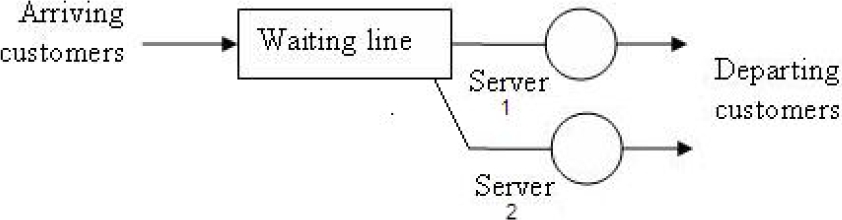
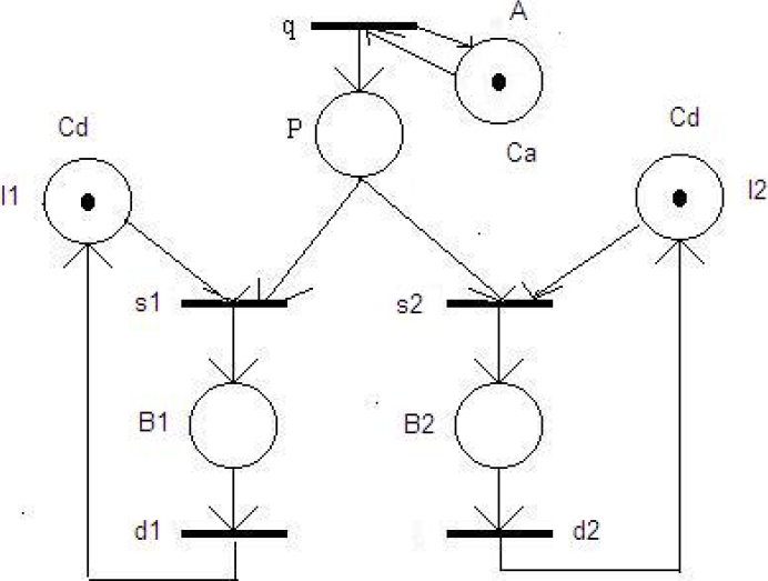
The places (that represent the states of the queue) are: A: customers arriving, P: the customers are waiting for service in the queue, B1, B2: the customer is being served, I1, I2: the servers are idle. The holding times associated to the places A and I1, I2 are Ca and Cd respectively, with Ca>>Cd.

The PN (TPN) is unbounded since by the repeated firing of q, the marking in P grows indefinitely. However, employing Lyapunov and Max-Plus algebra techniques, it has been shown that by taking u=[Ca,Ca/2,Ca/2,Ca/2,Ca/2]], the PN is stabilizable which implies that the TPN is stable i.e., the load has to be equally divided between the two servers [6].

We have already discussed a ψψ−−ASM whose program describes the dynamical behavior of a Petri net (see equation 20, equation (3)), therefore setting in our program m=6, t=5, and u=[Ca,Ca/2,Ca/2,Ca/2,Ca/2]], we are able to bound the marking in P or equivalently to avoid the unstable states of the queuing system i.e., the set Xun of our analog algorithm.

We conclude that by choosing properly the rules of the program ψψ−−ASM the analog algorithm for the two server queuing system is stabilizable.

4 Stability of Analog Algorithms in Terms of Lyapunov Energy Functions for Analog Algorithms with Continuous and Discontinuous States

In this section, we consider the stability concept for analog algorithms with continuous and discontinuous states in terms of Lyapunov energy functions. The results presented in this section, become a generalization of what was discussed in subsection 2.1 and section 3, and includes them as particular cases. It applies to many classes of discontinuous dynamical systems including hybrid systems and switched systems. We will deal with analog algorithms whose states are structures of vocabulary V, where now the the base set S is a metric space (S,d), with metric d.

Definition 30. Let us consider an analog algorithm, we will say that the state X, with a∈∈S and time-indexed location ft,t0(a), where t and t0 belong to T, is stable if and only if ∀∀t0∈∈T and ∀∀εε>>0  ∃∃  δδ=δδ(t0,εε)>>0 such that if given a′′∈∈S, with d(a′′,a)<δδ⇒⇒d(‖‖ft,t0(a′′)‖‖X,‖‖ft,t0(a)‖‖X)<εε  ∀∀t∈∈T.

Definition 31. Let us consider an analog algorithm, we will say that the state X, with a∈∈S and time-indexed location ft(a) is continuous at t∈∈T, if and only if ∀∀εε>>0  ∃∃δδ=δδ(t)>>0 and a state Y such that if given t′′∈∈T, with |t−−t′′|<δδ⇒⇒d(‖‖ft(a)‖‖X,‖‖ft′′(a)‖‖Y)<εε.

Definition 32. A continuous function αα:[0,∞∞)→→[0,∞∞) is said to belong to class K if it is strictly increasing and αα(0)=0.

Postulate E. The Lyapunov energy function associated to the analog algorithm at its starting time point t0∈∈T multiplied by some finite constant C≥≥1 bounds the whole Lyapunov energy function, transferred or transformed of the whole analog algorithm, as the Lyapunov energy function evolves in time.

Theorem 33.Let us consider an analog algorithm with the possibility of having discontinuous states at points {t1,t2,⋯⋯}⊆⊆T. Assume there exists a Lyapunov function V:S××T→→ℛℛ+ and two functions αα1, αα2, which belong to K, such that:

α1(dft,t0(a)X,ft,t0(a)XV(ft,t0(a)X,t)α2(dft,t0(a)X,ft,t0(a)X)),

for all a,a′′∈∈S,t,t0∈∈T. Assume Postulate E and that ‖‖ft0,t0(a′′)‖‖X=a′′ holds, then the analog algorithm is stable.

We want to show that there exists a δδ=δδ(t0,εε)>>0 such that given a′′ with d(a′′,a)<δδ⇒⇒d(‖‖ft,t0(a′′)‖‖X,‖‖ft,t0(a)‖‖X)<εε  ∀∀t∈∈T. Claim δδ=αα2−−1(C−−1αα1(εε)) does the job:

d(ft,t0(a)X,ft,t0(a)X)α11(V(ft,t0(a)X,t))α11(CV(ft0,t0(a)Xt0))=α11(CV(a,t0))α11(Cα2(d(a,a)))<ε.

Here postulate E has been used in the second inequality and the equation ‖‖ft0,t0(a′′)‖‖X=a′′ in the first equality.

It is worth mentioning that the preceding analysis applies to many classes of discontinuous dynamical systems, including hybrid systems and switched systems.

An example of a stable analog algorithm whose Lyapunov function satisfies the conditions imposed by theorem 33 is the one provided in [8], which consists of a ball in a constant gravitational field bouncing inelastically on a flat vibrating table. It is interesting to see how the Lyapunov function, proposed in the cited paper, monotonically decreases as t increases i.e., Postulate E holds with C=1.

Consider the switched system defined by the following scalar differential equation:

dx/dt={ln(2)xift[t0+2k,t0+2k+1],ln(4)xift[t0+2k+1,t0+2(k+1)],

where k∈∈N, x∈∈ℛℛ, and t0∈∈ℛℛ+. Then, taking V(X)=|X| as our Lyapunov function, all the conditions of theorem 33 with C=2 are satisfied, therefore concluding stability which implies that we get a stable analog algorithm.

5 Dynamical Systems with Non-Unique Trajectories

For continuous dynamical systems defined by differential ordinary differential equations, it is well-known that the continuity of the dynamical system does not guarantee uniqueness of solutions. Likewise, for discontinuous dynamical systems, uniqueness of solutions is not guaranteed in general, either no matter what notion of solution is chosen.

The lack of uniqueness of solutions generally requires a little bit of extra analysis because, we need to take into account the possibly multiple solutions starting from each initial condition.

This multiplicity leads us to consider the stability concept together with the adjectives total and partial. Roughly speaking, total is used when the stability property is satisfied for all solutions starting from each initial condition.

On the other hand, partial is used when the stability property is satisfied by at least solutions starting from each initial condition. Locally Lipschitz is the most common requirement invoked to guarantee uniqueness of solution.

Example 36. Consider the dynamical system defined by the following ordinary differential equation:

x(t)=[|x|]12,x,

which is continuous everywhere, and locally Lipschitz on ℛℛ\\{0}. This differential equation has two solutions starting from 0, namely: ϕϕ1:[0,∞∞)→→ℛℛ,ϕϕt1=0, and ϕϕ2:[0,∞∞)→→ℛℛ,ϕϕt2=t24.

Definition 37. An analog algorithm for non unique evolution operators is the Cartesian product of analog algorithms, where each one of the analog algorithms that belong to the Cartesian product satisfy all what was discussed in section 2.

Postulate E. An analog algorithm for non unique evolution operators is a dynamical system {T,X,A,{ϕϕti}i∈∈N}, where T, X, A are defined as in (2), {ϕϕti}i∈∈N is an indexed family of evolution operators parametrized by T, and for each i∈∈N fixed, there corresponds one member of the Cartesian product of analog algorithms.

Remark 38. From definition (37) by taking Cartesian products, it is immediate to generalize all the properties of analog algorithms, (given in section 2), to analog algorithms for non unique evolution operators, where now we have an ASM program associated to each one of the evolution operators and which defines the ASM program of the analog algorithm for non unique evolution operators.

Continuing with our previous example, the ASM program of the analog algorithm for non unique evolution operators that models it, turns out to be composed by the following two ASM programs:

if  True  then  ϕϕt1:=0,

if  True  then  ϕϕt2:=t224.

The set of updates is given by ΔΔψψ(X)={(ϕϕt1:=0)(ϕϕt2:=t224)}. Even more, the analog algorithm for non unique evolution operators results to be partially stable.

References

1.  1. Bournez, O., Dershowitz, N., Neron, P. (2016). Axiomatizing Analog Algorithms. [ Links ]

2.  2. Gurevich, Y. (2000). Sequential abstract-state machines capture sequential algorithms. ACM Trans Comput Log, Vol. 1. [ Links ]

3.  3. Retchkiman, K.Z., Dershowitz, N. (2019). The Church thesis, its proof, and the notion of stability and stabilization for analog algorithms. Communications in Applied Analysis, Vol. 23, No. 2. [ Links ]

4.  4. Murata, T. (1989). Petri nets: Properties, analysis, and applications. Proceedings of the IEEE, Vol. 77, pp. 541–580. [ Links ]

5.  5. Retchkiman, Z. (2005). Stability theory for a class of dynamical systems modeled with Petri nets. International Journal of Hybrid Systems, Vol. 4, No. 1. [ Links ]

6.  6. Retchkiman, Z. (2012). Timed Petri Net Modeling and Lyapunov/Max-Plus-Algebra Stability Analysis for a type of Queuing Systems by means of timed Petri nets, Lyapunov methods and max-plus algebra. International Journal of Pure and Applied Mathematics, Vol. 77 No. 3. [ Links ]

7.  7. Lakshmikantham, V., Matrosov, V.M., Sivasundaram, S. (1991). Vector Lyapunov functions and stability analysis of nonlinear systems. Kluwer Academic Publ. [ Links ]

8.  8. Heimsch, T.F., Leine, R.I. (2011). A novel Lyapunov-like method for the non-autonomous bouncing ball system. 7th European Nonlinear Dynamics Conference (ENOC). [ Links ]

Received: May 06, 2019; Accepted: April 20, 2020

* Corresponding author: Zvi Retchkiman Konigsberg, e-mail: mzvi@cic.ipn.mx

Creative Commons License This is an open-access article distributed under the terms of the Creative Commons Attribution License