


 text new page (beta)
 English (pdf)
 Article in xml format
 Article references
 Send this article by e-mail
 Cited by SciELO
  Similars in
SciELO
Similars in
SciELO 
 Permalink
1 Introduction
With the use of new technologies, the volume of bibliographic records generated is increasing. Daily, thousands of books, scientific papers, photos, videos and all kinds of materials are published in both digital and hard format. To facilitate the search and retrieval of information in this large volume of bibliographic records, metadata are used. Metadata are usually defined as ”data (information) about data” or ”data that define and describe other data”, [17, 18, 57, 74, 73]. For example, in the bibliographic resource book, the data is the book itself, while the metadata of the book is the author, the title, the publisher and other characteristics that describe the book. Like data, metadata quality is a crucial point of interest.
The term metadata quality is difficult to define [8]. Until now no consensus has been reached on its definition except for its multidimensional nature [76]. Agreeing [43], metadata quality can be defined similar to data quality, as ”fitness for use of data consumers”, [79, 10, 11, 72, 4, 70, 52, 82].
According to [77], data are described or analyzed through multiple dimensions, which are grouped in frameworks. These dimensions vary from one framework to another and depend on the context in which they are being analyzed [52]. Among the frameworks most referenced in the literature is the one proposed by [51], that identifies 23 quality parameters. However, some of these parameters (ease of use, ease of creation, protocols, etc.) are more focused on the metadata standard or metadata generation tools [59]. On the other hand, [34] proposed a framework presenting 21 quality dimensions grouped into three categories: intrinsic, relational/contextual and reputational. Some of the parameters (accuracy, naturalness, precision, etc.) are present in more than one dimension.
In Bruce and Hillmann’s framework [8], the problems that correspond to the quality of the metadata in libraries are analyzed and the dimensions proposed in [34] are grouped in seven general dimensions, independent of the domain with the aim of improving its applicability [73, 58, 59, 60]. These dimensions are completeness (Comp), accuracy (Accu), logical consistency and coherence (LCC), conformance to expectation (CoEx), accessibility (Acce), timeliness (Time) and provenance (Prov). This framework has been analyzed by several authors [28, 63, 75, 62, 16, 81, 45, 78, 64]. Table 1 shows the correspondence between its seven quality parameters and those proposed in other metadata quality frameworks in the period between 2009 and 2019.
Table 1 Correspondence between the Seven Dimensions of the Bruce and Hillman [8] Metadata Quality Framework and Several Frameworks of the last Ten Years
| Framework | Comp | Accu | LCC | Time | CoEx | Acce | Prov | Others |
| Ochoa and Duval, 2009 [60] | X | X | X | X | X | X | X | |
| Park, 2009 [63] | X | X | X | X | ||||
| Man, et.al., 2010 [44] | X | X | X | X | ||||
| Mendes et al., 2012 [49] | X | X | X | |||||
| Goovaerts and Leinders, 2012 [24] | X | |||||||
| Liaw et al., 2013 [35] | X | X | X | X | X | |||
| Palavitsinis, 2013 [61] | X | X | X | |||||
| Bellini and Nesi, 2013 [5] | X | X | X | |||||
| Tabares et.al., 2013 [75] | X | X | ||||||
| Tani et.al., 2013 [76] | X | X | ||||||
| Kemps-Snijders, 2014 [30] | X | X | X | X | X | X | X | |
| Palavitsinis et al., 2014 [62] | X | X | X | X | ||||
| Kiraly, 2015 [31] | X | X | X | X | X | X | X | |
| Alemu and Stevens, 2015 [1] | X | X | X | |||||
| Gavrilis et. al., 2015 [16] | X | X | X | X | ||||
| Zavalina et. al., 2016 [84] | X | X | X | |||||
| McMahon and Denaxas, 2016 [47] | X | X | X | X | X | |||
| Vaziri et. al., 2017 [69] | X | |||||||
| Kiraly and Buchler, 2018 [32] | X | X | ||||||
| Hopkinson et. al., 2018 [29] | X | |||||||
| Rashid et. al., 2019 [68] | X | X | X | X | ||||
| Cichy and Rass, 2019 [12] | X | X | X | X | X |
Within the quality dimensions proposed in [8], completeness, accuracy and consistency are the most used and, within them, completeness is the most used of all (see Table 1). In addition, incomplete metadata commonly affect the search and retrieval of information from them in digital repositories or online catalogs, due to the absence of basic elements [8, 56, 59]. Usually, this dimension is associated with the presence of incomplete fields in a record [6, 5]. According to Ochoa and Duval [58, 59, 60], in the case of metadata, completeness is defined as ”the degree to which a metadata record stores all the information necessary to have a global representation of the described object”.
This necessary information varies depending on the application domain and it is important to measure it in order to determine the level of completeness of a given record. In [58, 59, 60], two metrics are proposed for the completeness dimension. Specifically, the second metric is the weighted sum of the non-zero fields over the total sum of the weights of all fields. In this case, to calculate the weighting factor associated with each field, it is common to use the method based on the frequency of appearance of the fields in a given repository.
This method is considered inaccurate because its results depend on the quality of the cataloged metadata and this process is usually done manually, which is one of the most common causes of data quality errors [25]. In addition, it is expensive because weights must be recalculated as the volume of the repository grows. Therefore, the method used is not adequate and this paper aims to fill this gap by identifying the most appropriate method for estimating the weights for the completeness measurement of bibliographic metadata.
The rest of the paper is organized as follows. Section 2 briefly introduces the completeness metrics and the characteristics of the weighting factor, and discusses related works. Section 3 presents a comparative analysis about main methods for the weights estimation process, their strengths and weaknesses. Section 4 shows how the selected method was used. Section 5 presents and analyze the experimental results through a case study for MARC 21 format. Finally, section 6 concludes the study and provides directions for future research.
2 Related Work
In [58, 59, 60], several metrics are suggested for each dimension of Bruce and Hillman’s framework [8], which complements it. Those metrics have been retaken in works such as [21, 31, 19, 32]. Specifically, for the completeness dimension, the following metrics are proposed: A basic metric that consists of counting the number of fields in each case of the metadata that contain a no-null value. Equation 1 expresses how this metric can be determined [58, 59, 60]:
where N represents the number of fields defined in the metadata standard, and P(i) takes value 1 if the ith field has a no-null value, 0 otherwise.
This completeness metric does not reflect how users measure completeness because not all elements of metadata are equally relevant in all contexts. For example, a human expert may assign a higher degree of completeness to a case that has title, but lacks the publication date and vice versa.
To explain this phenomenon, Ochoa and Duval [58, 59, 60] introduce a weighting factor that is multiplied by the presence or absence of a given field. This factor represents the importance of the field and can be easily included in the calculation of completeness, as expressed in equation 2, and it is also known as weighted metric:
where αi means the weight factor or degree of importance of the ith field. In addition, equation 1 is a particular case of equation 2 where all the fields have a degree of importance equal to 1.
In both metrics, when there is more than one case in a field, this field is complete if at least one of its cases is complete. By measuring the completeness of a record with these metrics, we can know how complete are the stored data respect to the used metadata format.
According to the characteristics of the weighted metric expressed in equation 2, a weight or importance degree is assigned to each field. These weights are usually different numerical values for each field.
It is known that there are fields more important than others, for example thematic fields, title, author and year of publication are the most frequently used in search engines such as Google, Google Scholar, IEEE Xplore, CiteSeerX, Web of Science, SCOPUS, among others to retrieve information or quote an article.
In the last case, when a reference or bibliographic citation is created, usually not all the fields are filled, often because the data is not available or because it simply does not interest to be considered as a valid reference, for example the abstract and tags fields are rarely filled up, despite their usefulness.
On the other hand, there are stable formats that are more complex, such as the Machine Readable Cataloging (MARC 21) format for bibliographic records. Each record can describe one of the following eight classes of materials: book, computer file, score, map, serial publication, mixed material, sound recording and visual material [2].
In addition, there are three cataloging levels: minimal [38], full [37] and general [42]. In these levels, the fields that belong to the general level contain those of the full level and other fields. Those of the full level contain those of the minimal level and other fields, and so on, being the minimal level the one that contains a subset of essential fields for cataloging.
In a first approach, inspired by this behavior, we can create importance levels to assign the weights to the fields. In this way, the final values will be closer to what actually happens. This work allows creating as many levels as needed to estimate the weights and the way to calculate them varies depending on the criteria of the specialists or the result of other investigations.
For example, in [48] from the analysis of 69 Spanish metadata repositories, it was detected that the title, identifier, date, language, format, description, type and subject fields are the eight most used Dublin Core fields. In cases where this division by levels does not make sense because the metadata format is very simple or because it is not necessary, we assumed that there is a single importance level for all fields, and therefore, equation 1 applies.
3 Methods for Estimating Weights
The algorithm to calculate the completeness metrics needs access to the metadata repository and, in the case of the weighted metric, also requires a table containing the values of the weights αi calculated. In equation 2, the authors do not define the values for the parameter αi, which depend on the context in which they are used. In this paper, it is assumed as a criterion that the values of αi are continuous, included in the interval (0, 1) and
In the consulted literature, there are different methods for calculating the weights αi. In this section, we analyze the strengths and weaknesses of the selected methods for weights estimation with the purpose of selecting the most feasible according to the problem covered in this research. In addition, comparison parameters are established.
3.1 Method based on the Appearance Frequency of the Fields
In [60], from the frequency of use of the fields in searches to the ARIADNE repository as reported in [53], the alphas needed in equation 2 were obtained. For example, αi represents the number of times field i has been used in queries to a given repository.
Another variant similar to the previous one is the proposal in [20], where the weights are calculated as the sum of the incidences (appearance frequency) of each field in a set of records with the same material class, such as books, mixed materials, among others. The incidence of a field in a record consists of the absence or presence of a field within it [46]. Additional to the previous definition, the field must be complete in order to influence a record. In order to obtain the degree of importance of a given field, in [20], the equation 3 is proposed:
where N represents the number of records, R(j) takes value 1 if field i is present and complete in the jth record, and 0 otherwise. The completeness of the field gives the incidence of a field in a record. Using equation 4, the weight of each field per material class is then calculated:
where αi represents the weight of the normalized ith field in the interval (0, 1). F Ai the appearance frequency of the field ith in the type of current material and F AT the sum of the F Ai belonging to this material.
In spite of the simplicity of its calculation, this method presents disadvantages because the calculated weights depend on the data repository and therefore on their quality. If there are records within the repository that their metadata are incorrectly cataloged, then the fields receive incorrect weights. This is because the method assigns more weight to the most used fields and gives zero to those that are not used within the analyzed repository. In addition, if the repository change, we must recalculate the weights, which adds additional cost to the execution time. This time is proportional to the volume of the repository.
3.2 Exact Solution Methods
Exact solution methods such as simplex, gradient method, Newton-Raphson method and transport model provide optimal value in a search space that may or may not be restricted. These methods locate the exact value of the search space that represents the optimal of the objective function stated in the mathematical model being solved. Some of the main advantages of the exact solution methods are:
— They always converge to a feasible solution that represents the optimum of the search space, if it exists.
— They have few parameters to adjust and they need little memory for their execution.
However, exact methods are not always the right way. These manifest several disadvantages that make it difficult to use them in many reality problems.
In [50], the authors argue the reason for the existence of so many exact methods can correspond to the fact that none of these can apply to a great variety of problems. This is due to the peculiarities of the problem in question, which may make it impossible to use certain exact methods and with it arises the need to create others that correspond to the problem posed. Nevertheless, there are problems that cannot be solved because of their complexity or the large size of their search space, such as problems of the NP-Complete type, where the search for a solution becomes too slow. The time required to reach a solution is proportional to the number of variables and the size of the search space.
At the same time, the knowledge of the problem modeled manifest through the restrictions imposed on the model, which helps to reduce the exploration, and allows finding the solution in a shorter time. Nevertheless, problems do not always have a solution in an acceptable time. Regarding this situation, using heuristic procedures to find a good suboptimal solution is preferred by specialists. This occurs most often when the time or cost required to find an optimal solution for a suitable model of the problem would be very large. In recent years, great progress has been made in developing efficient and effective metaheuristics that provide both, a general structure and strategic guidelines for designing a specific heuristic procedure to fit a particular kind of problem [27].
3.3 Genetic Algorithms (GA)
GAs are inspired by the nature and function as a stochastic model. The GA has the ability to solve a variety of very difficult problems such as working without prior knowledge of the function to be optimized, working without secondary information, for example, gradients and optimizing ”noisy” functions.
Most specialists agree that GAs can solve the difficulties represented in real-life problems that sometimes are insoluble by other methods. According to [22], the central theme of research at the GA is robustness, the balance between effectiveness and efficiency needed to survive in different environments. [23] also highlights the ways in which GAs differ from traditional systems:
— They work with a coding of the parameter set, not with the parameters themselves.
— They search from a population of points, not from a single point.
— They use only information from the objective function, without derivatives or other auxiliary knowledge.
— They use probabilistic, not deterministic transition rules.
In addition, [23] expressed some of the reasons why GAs can be appealing for application development:
— They make possible to solve difficult problems quickly and reliably.
— They are easy to link to existing simulations and models.
— They are extensible.
— They are easy to hybridize.
However, GAs offer no guarantee of convergence on arbitrary problems. They quickly sort interesting areas of a space, but are a weak method, without the guarantees of more convergent procedures. In this case, it is better to use local methods instead of convergent ones. The solution is to apply a hybrid scheme. Therefore, we can combine the globality and parallelism of the GA with the convergent behavior. At a given time, all individuals in the population have a very close adaptation or adjustment value and little improvement from one generation to the next one. If at the beginning of a run, the selection operator takes a significant proportion of the population in a generation, it may lead to premature convergence. At the end of a run, the average population adjustment may be close to the best population adjustment; this may lead to random movement among the mediocre individuals [23].
Other difficulties detected in the work with GA that have led researchers to deepen in theoretical aspects are:
3.4 Particle Swarm Optimization (PSO)
There are problems where classic optimization algorithms fail to provide an optimal global solution, arriving only at local solutions or that the computation time needed to respond is very high. To deal with these types of complications, optimization algorithms such as PSO are applied. PSO is a very effective algorithm, with only the value of the objective function and without the need for any extra information such as the gradient or the size of the search space, quickly finds feasible solutions very close to the overall optimum [7].
This metaheuristic is also inspired by the nature and function as a stochastic model. It is easy to implement and hybridize with few parameters to adjust and it is an advantageous tool for solving problems of various kinds such as:
— Optimization of functions.
— Training of artificial neural networks.
— Fuzzy control systems.
— Estimation of parameters for other meta-heuristics.
The main disadvantage that PSO has is the correct calculation of the velocity either by limiting it between [-Vmax, Vmax]], applying a decreasing dynamic inertia coefficient or applying the constriction coefficient to the velocity before updating the position of the particle relative to it. Two cases may occur, the first where the velocity values are small, and then premature convergence to local optimal generally occurs due to poor exploration of the search space. The second case is the other way around, when the values are very large and it is possible to exceed promising regions that represent optimal solutions and not consider them to give answer to the optimization problem posed.
3.5 Comparison between Methods for Estimating Weights
Table 2 compares the four methods presented in Sections 3.1 to 3.4, in terms of five selection criteria that help to determine what method is more feasible for estimating weights.
Table 2 Comparison between Analyzed Methods for Estimating Weights
| Features\Methods | AppearanceFrequency | Exact Methods | GA | PSO |
| Type of variable | Continuous | ContinuousDiscreteBinary | ContinuousDiscreteBinary | Continuous |
| Degraded performance with more than 100 variables | Yes | Yes | No | No |
| The completeness of the cataloged records influences the estimation of the degree of importance of each field | Yes | No | No | No |
| Weights recalculation if the volume of the repository grows | Yes | No | No | No |
| Number of parameters to define | None | Depends on the method | Four or more | Two |
The first criterion, presented in Table 2, refers to the type of variable. According to the literature, the PSO method has a better performance to treat continuous variables [26, 15, 67], and the type corresponding to the weights (αi) is precisely continuous.
Regarding the second criterion, in the exact methods, the execution time is proportional to the number of variables involved in the solution, which makes them less effective. In addition, there is a direct relationship between the number of variables and the number of fields allowed by the analyzed bibliographic metadata format. In cases where the formats have more than 100 fields, these methods collapse. For example, the MARC 21 format has 999 fields and 281 fields for bibliographic records, the Text Encoding Initiative (TEI) [9] format has nearly 500 elements, and the Encoded Archival Description (EAD) [41] tag set has 146 elements.
However, the execution time is not affected in metaheuristics, because these randomly chosen regions of the search space, whether good or bad, after successive and quickly iterations, improve solutions, and return values very close to the optimum. The number of iterations is directly proportional to the degree of specialization of the solutions found.
The third criterion refers to whether or not the completeness of records already cataloged influences in determining the degree of importance of each field. In the case of the method based on the appearance frequency of the fields, it does influence because this method is counting, record by record, the fields that are complete and the rest of the fields are not taken into account. This causes incorrect weights to be assigned to the fields at the end.
For example, if, in certain records, the title field is not cataloged (although it actually exists), this field will be assigned a low weight by this method, even though it is known that the title is one of the fields by which searches are made to retrieve information. On the other hand, it may happen that a field that is not really so important is introduced and then assigned a high weight. This commonly happens because this method depends on the quality with which the specialist has cataloged each record (the data itself). This is not the case with the rest of the methods, compared in Table 2, that depend only on the structure (metadata format).
The fourth criterion refers to whether it is mandatory to recalculate the weights of the fields as the volume of the records cataloged in the repository grows. In the case of the method based on the appearance frequency of the fields, this is fulfilled, because the frequency changes as the volume of repository data and cataloged records changes, and therefore, the calculated weights also change. In summary, the third and fourth criteria highlight the main disadvantages of the method based on the appearance frequency of the fields regarding the rest of the methods compared.
PSO and GAs share some similar characteristics, for instance, both methods begin their processes from randomly generated populations that do not require any input from user. PSO and GAs need to establish initial parameters such as chromosome for GAs and particle for PSO, the number of generations, population size in GAs, or amount of particles in PSO. However, the last selection criterion in Table 2 highlights that GAs need to define more parameters than PSO. The parameters are crossover probability, type of crossing (one point, two points, uniform, etc.), probability of mutation and type of selection. Choosing the type of selection is also challenging because there are several selection techniques such as roulette wheel selection, rank selection, tournament selection, steady state selection, Boltzmann selection and elitist selection [80, 71].
In addition, the chosen selection technique can define other parameters, like expressed in [80, 71]. While PSO only needs to define two parameters, the velocity vector and the constriction coefficient. In [67], the authors analyzed the operators of GAs and PSO and concluded that PSO is more efficient and accurate than GAs. According to the authors in [26], ”PSO outperforms the GA with a larger differential in computational efficiency when used to solve unconstrained nonlinear problems with continuous design variables”.
In addition, in [15], the authors argue that the main disadvantage of GAs is that its solutions can be trapped in local optimum. This is because it does not take into account the best overall position of the individual.
Such drawback is overcome with the PSO technique, which tracks the best individual position of the particle, as well as the best global position, therefore, it moves towards a global optimum without being trapped in the local optimum. PSO exceeds GA and is more effective overall, however, the superiority of PSO depends on the problem.
[66] affirms that the experimental results of [3] show that PSO algorithms not only converge faster but also run faster than GA. For more information on this comparative analysis between GAs and PSO, see [26, 15, 3, 67, 66].
4 Particle Swarm Optimization Method for Weights Estimation in Bibliographic Metadata
In the PSO method, each particle (individual) is a vector that represents a position in the search space and it is associated with two vectors.
The first one represents the velocity and direction of displacement, while the second one is a copy of the best solution found in its movement. The position defines the content of a candidate solution and possesses a quality measure.
A particle can interact with a number of neighbors [7], whose value and position it knows. Implementing the principle of comparing and imitating, it learns, adjusting its position and velocity. The particle is partially attracted to a position between the best solution found in the course of its displacement (cognitive learning) and the best found by its neighbors (social learning).
This communication between them is called collective intelligence, also defined as a structured collection of interacting organisms (or individuals). Intelligence is in the collective. Each individual follows simple rules, but the collective executes complex tasks and no member controls the group.
4.1 Velocity Vector
Each of the particles (or individuals) in the swarm has an associated velocity vector, which determines its speed and direction of movement in the search space. To calculate velocity, equation 5 is used, with the sum of three parts:
The first part is the previous velocity of the particle Vi multiplied by a real value w known as inertia. The parameter w varies in the interval (0,1) and controls the impact of the historical velocity on the current velocity [83]. Large values facilitate global exploration, while small values facilitate local exploration. The second part is the difference between the best position found by the particle XP Besti, and the current position Xi.
This cognitive part represents learning from its own experience (c1). The last part is the difference between the best position reached by a neighbor XGBest, and the current position of the particle. This is the social part (c2), which represents the learning of the group. Parameters c1 and c2 with low values allow exploring different regions before heading for the target, while higher values allow sudden jumps to the target. According to [54], the recommended values are those that satisfy c1+c2 ≤ 4.1 as c1 = c2 = 1.4961 or c1 = c2 = 2.05.
A common problem with PSO algorithms is that the magnitude of velocity tends to become very large during execution, causing particles to move too fast in space. In [65], they state that performance may decrease if the value of the initial maximum velocity of each component of the velocity vector (Vmax) is not properly set. If the velocity of a particle is greater than Vmax, it can surpass good solutions.
On the other hand, if it is less than -Vmax, it can fall into local optimal because there is not enough exploration beyond locally good regions. The two methods proposed to control the excessive growth of the velocities are:
— An inertia factor (w), dynamically adjusted. An adequate value produces a balance between global and local search [55]. In addition, it reduces the number of generations required and recommends a high initial value and a gradual decrease; this allows a global search at the beginning and a local search to the end.
— A constriction coefficient (k), this value multiplies the velocity vector obtained in equation 5 and ensures convergence to the best solutions faster [13]. Equation 6 is used for its calculation, where ϕ = c1 + c2 > 4:
In this work, we implement PSO method with the modifications in the calculation of velocity proposed in [55], to avoid premature convergence. Further, we describe the rest of the components of the algorithm as follows.
4.2 Fitness Function
Equation 7 shows how to measure the fitness of a solution:
where
— n represents the number of importance levels, at which the fields can be grouped,
— mi signifies the number of fields at the ith level,
— wi is the weight of the ith level, which is calculated using equation 8,
— P (i, j) is a function that returns the degree of importance associated with the ith field of the jth level in the current solution. The value of P (i, j) varies in the interval (0, 1) and
and
4.3 Model Restrictions
— The solution vector is a descending ordered sequence of numbers greater than zero and less than one.
— The sum of the components of the solution vector is strictly equal to one.
These two restrictions allow PSO searching for solutions in a much smaller search space than the interval (−∞, +∞). Calculation of velocity Equation 5 uses a dynamic w, whose initial value is 0.9 and gradually descends to 0.4, parameters c1 and c2 have equal value of 2. Then, using equation 6, the constriction coefficient multiplies the velocity vector, where the values of c1 and c2 are equal to 2.05.
5 Measurement of the Completeness of Bibliographic Records in MARC 21 Format: A Case Study
PSO method is valid to apply in the estimation of the weights of the fields of any metadata format. However, we decided to start by the MARC 21 format for bibliographic data as a case study, because in the cataloging module of the ABCD software suite for the automation of libraries and documentation centers of the Cuban universities that belong to the VLIR ICT Network, there are incomplete bibliographic records. Something similar occur in the catalog of the Library of Congress. Although it is not known with certainty how serious the problem is. In addition, MARC 21 is currently the most widely used coding format for transferring bibliographic information, prestigious libraries and documentation centers in countries such as Brazil, Belgium, the United States (Library of Congress) and Cuba, use it.
MARC 21 clearly illustrates the levels of importance of the fields, and it is one of the most complex formats for the description of bibliographic records. MARC 21 for bibliographic records is designed to contain bibliographic information, such as titles, names, subjects, notes, publication information, and physical description of items [2]. It contains data elements for the following eight classes of materials: books, continuous resources, computer files, maps, music, sound recordings, visual materials, and mixed materials. Three main elements, the header, the directory and the variable fields, form a record in this format [39]:
— Header: contains information needed to process the record.
— Directory: several entries indicating the label, length and starting point of each variable field.
— Variable fields: these can be of two types: control variable fields and data variable fields.
— Data variable fields are composed of indicators and subfields.
— Control variable fields provide coded information about the record as a whole and about special aspects.
To determine whether a field belonging to the MARC 21 format is complete raised the following considerations:
— A case of a variable field of a record is complete if:
— Its value is not the empty string, in the case of control variable fields.
— Its value is not the empty string, if at least the subfield a is present, in the case of data variable fields.
— A variable field is complete if at least one of its cases is complete.
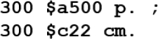
Figure 1 shows two cases of the repeatable variable data field with label 300 referring to the physical description of the analyzed item. According to the previous considerations, field 300 is complete because at least one of its cases is complete, since the first case is complete because it presents subfield a and its value is not the empty string.
5.1 Importance Levels of the MARC 21 Fields
The number of importance levels varies from one format to another, and from one country to another. For example, as a first approach, in MARC 21 format for bibliographic records, initially three levels of importance group the fields, one by each cataloging level of each material class: minimum, full and general. Where the fields belonging to the minimum level are the most important ones, those concerning the full level, the second in importance, and finally those belonging to the general level.
According to MARC 21 Format for Bibliographic Data Field List there are 281 fields, but we dismiss the fields 090, 091 and 590 because they are used for local use, and the fields 251, 341, 532 and 758 because they are for special resources. Therefore, we consider 274 as the total number of fields for bibliographic records in the general level. Note that there are seven fields in the minimal level that are mandatory for all material classes, those fields are 001, 003, 005, 008, 040, 245 and 300 [40]. This way, the distribution of the fields stays for each material class according to the three levels of importance mentioned. It is assumed that the sum of the weights of level one is greater than that of level two and so on.
On the other hand, consideration is given to the criteria of specialists, who may establish the number of importance levels according to their expertise in working with the format. We create a software to generate the weights according to the number of importance levels, the distribution of the fields by each level, the number of generations, the number of particles provided by the specialist.
But, we also provided default values for each parameter. Those default values are the results of several running of the PSO algorithm in the case of the number of generations and number of particles, and the results of a questionnaire applied to seven specialists in MARC 21 format, in the case of the number of importance levels and the distribution of each field by importance level. These questionnaire was designed for the eight material classes in MARC 21 for bibliographic records at the full cataloging level to simplify the process.
The composition of these specialists was as follows: all are university graduates, six are from Cuba and one from Belgium, three have a PhD degree, two have a Master degree and one is a specialist. According to their working experience, six have ten or more years and one between six and nine years of experience. Regarding their experience with the use of MARC 21 format, two have ten or more years, one between seven and nine years and four between four and six years.
All the specialists know the MARC 21 fields, four of them have developed application that used this format, three of them have taught courses about MARC 21 and three of them have worked in the evaluation of the metadata quality in general. In relation to the publications in journals or conferences, two specialist have five or more papers, one of them have three papers, another has two papers and another have one paper. According to the above aspects, we calculate the competition coefficient K for each specialist. This coefficient allows classifying them as follows:
Another rank could be taken for classification, but the one expressed in [14] was followed. Thus, there are three specialists with high competition and four with average competition.
To determine the coincidence (consensus) of the specialists in their voting, the Kendall rank concordance coefficient is used [14], see equation 9:
where
and
— n represents the number of items,
— k is the number of specialists or experts,
— Rj signifies the sum of values per column,
—
We use the procedure proposed in [33] for the design and application of the interview, but in our case to MARC 21 specialists:
Bibliographic review: from the review of the specialized literature in bibliographic metadata with MARC 21 format, an initial interview proposal is made on the degree of importance attributed to each field of the full cataloging level,
Content analysis: the content of the interview is validated using specialists from libraries and documentation centers, selected with non-probabilistic sampling intentional, and these variables are taken into account: language, adaptation to the factors, understanding of the questions and completeness measures. The range is 1 to 5. The Kendall Concordance Coefficient is calculated, being 0.96 for the class of Book material, 0.95 for the class of Score material and 0.99, for the rest of the material classes, thus it is high in all cases.
The coefficient of variability per item in each material class was also calculated. Lower percentages of variability mean that the experts responses do not differ much. As it turns out, in books, maps and scores, the coefficients are below 25%, in computer files, they are below 20%, in serial publications and visual materials, below 30%, in mixed materials, below 22% and in sound recordings, below 16%.
Taking these values and the calculated Kendall coefficients into account, it is shown that there is a low variability per item (between 16% and 30%) and high consensus among specialists (0.95 or more). Therefore, it is decided to select mode as a central tendency criterion to establish the importance levels of the fields according to their bibliographic material class. The final results are presented in Table 3.
Table 3 Distribution of the Fields for each Material Class into Importance Levels at the Full Cataloging Level
| Material Class(# Fields) | High Level | Medium Level | Low Level |
| Book (16) | 001, 003, 005, 008, 040, 082, 100, 245, 246, 260, 300, 650 | 007, 020, 500 | 050 |
| Computer File (16) | 001, 003, 005, 008, 040, 100, 245, 256, 260, 300 | 250, 500, 520, 538, 710, 753 | - |
| Score (13) | 001, 003, 005, 008, 040, 100, 245, 260, 300, 650 | 028, 240, 710 | - |
| Map (20) | 001, 003, 005, 008, 034, 040, 100, 245, 255, 300, 650 | 007, 052, 110, 246, 500, 700, 710, 730 | 260 |
| Serial Publication (25) | 001, 003, 005, 008, 035, 040, 210, 222, 245, 246, 260, 300, 310, 650 | 010, 022, 042, 043, 050, 082, 362, 500, 710, 780, 850 | - |
| Mixed Material (29) | 001, 003, 005, 008, 040, 100, 245, 300, 650 | 007, 010, 035, 041, 506, 520, 524, 555, 600, 610, 651, 655, 656, 852 | 351, 530, 541, 544, 545, 546 |
| Sound Recording (21) | 001, 003, 005, 008, 040, 100, 245, 260, 300, 650 | 007, 028, 043, 045, 047, 048, 050, 500, 511, 700 | 505 |
| Visual Material (24) | 001, 003, 005, 008, 040, 245, 300, 650 | 007, 033, 043, 050, 082, 246, 260, 440, 500, 508, 518, 520, 521, 651, 700, 710 | - |
5.2 Application of the PSO Method in the Calculation of Weights and the Completeness Measurement for the MARC 21 Format
In the experiments, we extracted by chance, the first 12 records from the official catalog of the Library of Congress [36], called R1, R2 · · · R12. Those records match in the advanced search with the word Freedom, the material class Book and the language English.
Table 4 presents the fields of the full cataloging level of the 12 records of the case study. In addition, Table 4 shows the completeness measurement of the selected bibliographic records using the weights estimated with the PSO method proposed at full cataloging level. PSO was running with 50 generations and 200 particles, and the distribution of fields per importance level according to Table 3.
Table 4 Example of the Calculation of Weights using the PSO Method Proposed and Completeness Measurement at Full Cataloging Level for Books
| Field | R1 | R2 | R3 | R4 | R5 | R6 | R7 | R8 | R9 | R10 | R11 | R12 | Weight |
| 001 | X | X | X | X | X | X | X | X | X | X | X | X | 0.1885 |
| 003 | - | - | - | - | - | - | - | - | - | - | - | - | 0.1631 |
| 005 | X | X | X | X | X | X | X | X | X | X | X | X | 0.1456 |
| 007 | - | - | - | - | - | - | - | - | - | - | - | - | 5.6E-5 |
| 008 | X | X | X | X | X | X | X | X | X | X | X | X | 0.1380 |
| 020 | X | X | X | X | X | X | X | X | X | X | X | X | 4.9E-5 |
| 040 | X | X | X | X | X | X | X | X | X | X | X | X | 0.1123 |
| 050 | - | X | X | X | X | X | X | X | X | X | X | X | 1.1E-16 |
| 082 | - | - | - | X | X | X | X | X | X | X | X | X | 0.0865 |
| 100 | X | X | X | - | X | X | X | X | X | X | X | - | 0.08020 |
| 245 | X | X | X | X | X | X | X | X | X | X | X | X | 0.03866 |
| 246 | - | X | - | - | - | - | - | - | - | - | - | - | 0.0288 |
| 260 | - | - | - | - | - | - | - | - | - | - | - | - | 0.0157 |
| 300 | X | X | X | X | X | X | X | X | X | X | X | X | 0.0021 |
| 500 | - | - | X | - | - | X | - | - | X | - | - | - | 2.8E-5 |
| 650 | - | X | X | X | X | X | X | X | X | X | X | X | 3.8E-4 |
| TFF | 8 | 11 | 11 | 10 | 11 | 12 | 11 | 11 | 12 | 11 | 11 | 10 | |
| Comp | 0.705 | 0.734 | 0.705 | 0.712 | 0.792 | 0.792 | 0.792 | 0.792 | 0.792 | 0.792 | 0.792 | 0.712 |
The fields shown in Table 4 correspond to the full cataloging level in the material class “Book” (16 fields). The weights were calculated using these fields to illustrate the proposed method, therefore, if there exist other fields, it is assumed that they have zero degree of importance (zero weight). In the completeness computing of each record, we used the weighted metric presented in equation 2. The results approximate up to four decimal places after the decimal point in the calculation of the weights, and three places in the case of the completeness measurement, just to illustrate the results. In addition, TFF refers to the Total Fields Filled in each record.
In Table 4, fields 003 (control number identifier), 007 (fixed field of physical description) and 260 (publication, distribution, etc. (imprint) ) are always empty in the 12 bibliographic records analyzed. Specially 003 is a mandatory control field for all classes of materials. In addition, the record R2 is the only one with the field 246 (varying form of tittle), in the other 11 records, this is missing. On the other hand, the most complete records are R6 and R9 with 12 out of the 16 total fields. All the completeness values are between 0.7 and 0.79, which is considered medium-high. These completeness values indicate that records have the majority of the most important fields completed, but still need to be reviewed to improve the incomplete fields, such as mentioned above.
The decision to present the results at the full cataloging level was to simplify the process and because the records are generally cataloged up to this level. This is not the case with the general level, because it is difficult to find records with all 274 fields that make up this level filled in.
However, it is very similar to do this way with the general cataloging level, for example you can add another importance level with the rest of the fields and run again the PSO method proposed. In addition, the completeness metric is sensitive to the number of fields, the larger the total number of fields, probably smaller the value of the measure of completeness calculated.
In this way, the completeness values obtained in Table 4 are closer to one in the measure that the most important fields are present and closer to zero otherwise.
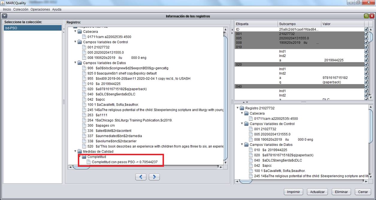
This is because of the creation of importance levels between the fields. The estimated weights do not depend on the quality of the bibliographic records cataloged nor the repository employed. Figure 2 shows part of the MARCQuality tool with the description of the record R1 and the measurement of the completeness of the record R1 with the weights estimated by the PSO method proposed.
6 Conclusions and Future Work
The comparative analysis carried out revealed that the PSO method is the most robust one for estimating weights in the completeness measurement of bibliographic metadata. PSO adapts to different scenarios, it is very easy to implement and it offers multiple solutions that are built randomly and gradually, these are refined and improved, concentrating on points in the search space that are close to the global optimal. For using the PSO method, in the weights estimation for the completeness metric in different metadata formats, it is only necessary to vary the number of fields, the fields themselves, the number of importance levels and the field distribution per each importance level, because the model and the restrictions remain unchanged.
To measure the completeness of each bibliographic record in a repository, it is only required to apply the weighted completeness metric because the weights were previously calculated. The estimated weights are independent of the repository and, therefore, of the quality of the cataloged metadata, thanks to the characteristics of the PSO method proposed. In addition, those weights and therefore the completeness values are closer to reality due to seven specialists with high consensus among them, defined importance levels for each field by bibliographic material class at the full cataloging level in MARC 21 format.
In future works, we will analyze different ways to improve the completeness of the bibliographic records in several catalogs for different classes of materials. In addition, research must continue on other dimensions such as accuracy and consistency to improve the overall quality of bibliographic metadata.

