1 Introduction

In this paper the notion of discrete time event algo-rithms is introduced. The paper starts proposing a formalization, free of any interpretation, of discrete event time algorithms, and continues discussing computability issues. A Church type thesis, its proof, and the notion of stability for discrete event time algorithms are proposed.

The Church thesis for discrete algorithms motivates us to consider the Church thesis for the case when we are dealing with discrete event time algorithms. Gurevich [¹] has shown that any algorithm that satisfies three postulates can be step-by-step emulated by an abstract state machine (ASM). Adding two more postulates, Dershowitz and Gurevich [²] proceeded to prove that all notions of algorithms for common discrete-time models of computation in computer science are covered by this formalization.

This includes Turing machines, Minsky counter machines, Post machines, random access memory (RAM) and so on. Bournez, Dershowitz and Neron [³] have formalized a generic notion of analog algorithm, their proposed framework is an extension of [¹, ²]. They provide postulates defining analog algorithms in the spirit of those given for discrete algorithms, and continue proving some completeness results. Our presentation follows a similar construction to the one given for analog algorithms.

The notions of discrete event time algorithm and discrete event time dynamical system are postulated to be equivalent. The stability concept for discrete event time algorithms is defined. The stability analysis presentation starts concentrating in discrete event time algorithms i.e., discrete event time dynamical systems, whose Petri net model is described by difference equations, and continues considering Lyapunov energy functions in terms of the logical structures of the vocabulary.

A stability analysis based on the reachability tree of the Petri net model is also discussed. The paper is organized as follows. In section 2, axiomatization and computability issues related to discrete event time algorithms are presented. Section 3, discusses the stability problem for discrete event time algorithms in terms of its equivalent discrete event time dynamical system. Section 4 presents an application example. Section 5 discusses the states, (equivalently strucures), stability problem for discrete event time algorithms in terms of Lyapunov energy functions, and finally in section 6, a stability analysis based on the reachability tree is also discussed.

2 Discrete Event Time Algorithms, the Church Thesis

Gurevich [¹] has shown that any algorithm that satisfies three postulates can be step-by-step emulated by an abstract state machine (ASM). Adding two more postulates, Dershowitz and Gurevich [²] proceeded to prove that all notions of algorithms for common discrete-time models of computation in computer science are covered by this formalization. Bournez, Dershowitz and Neron [³] have formalized a generic notion of analog algorithm, their proposed framework is an extension of [¹, ²].

They provide postulates defining analog algo-rithms in the spirit of those given for discrete algorithms, and continue proving some completeness results. The next presentation follows a similar construction to the one given for analog algorithms, adapting it for discrete event time algorithms. In this section the formalization, free of any interpretation, of the notion of discrete event time algorithm as well as a Church type thesis based on the previous cited work are presented.

The reader looking for a more detailed discussion of the ideas behind the following presentation is encouraged to review [¹, ², ³] but in particular [¹] is recommended.

Definition 1 A dynamical system is a four-tuple {T, X, A, φ_t}, where T is called the time set, X is a state space, A is the set of initial states A ⊂ X and φ_t: X → X is a family of evolution operators parameterized by t ∈ T satisfying the following properties: for x ∈ X, φ₀(x) = x, and φ_t+s = φ_t◦φ_s.

Remark 2 Note that in our definition of dynamical system, it is allowed to have, in general, more than one evolution operator.

When T = N = {0, 1, 2, · · · } we speak of a discrete event time dynamical system. We will consider T equipped with the absolute value as a normed space i.e., (T, | · |) . A discrete event time dynamical system is generally represented by difference equations.

Remark 3 When dealing with discrete event time dynamical systems determined by difference equations on ℛn, we define the euclidean metric d as: d(x,y)=|x−y|=[∑i=1n(xi−yi)2]12,∀x,y∈ℛn. X equipped with the above euclidean metric defines a metric space.

Definition 4 A discrete event time dynamical system is said to be computable if and only if its family of evolution operators (also called its trajectories) is obtained as solutions of its mathematical model.

Postulate A. A discrete event time algorithm is a discrete event time dynamical system.

Definition 5 A vocabulary V is a finite collection of fixed-arity (possibly nullary) function symbols. We assume that V contains the scalar (nullary) function true. A first-order structure X of vocabulary V is a non-empty set S, the base set (domain) of X, together with interpretations of the function symbols in V over S, denoted by ‖f‖X. Similarly, the interpretation of a term f(t₁, · · · , t_n) in X is recursively defined by ‖f(t1,⋯,tn)‖X=‖f‖X(‖t1‖X,⋯,‖tn‖X). Let X and Y be structures of the same vocabulary V. An isomorphism from X onto Y is a one-to-one function ζ from the base set of X onto the base set of Y such that f(ζt₁, · · · , ζt_n)) = ζ(t₀) in Y whenever f(t₁, · · · , t_n) = t₀ in X.

Definition 6 A state transition system, consists of a set of states S, a subset I of initial states, transition functions on states, which determines the next-state relation, (states with no “next” state, will be terminal states).

Postulate B (Abstract state). States are first order structures with equality, sharing the same fixed, finite vocabulary. States and initial states are closed under isomorphism. Transitions preserve the domain, and transitions and isomorphisms commute.

Remark 7 In more simple words, states are structures which are invariant under isomorphism, and as a consequence they result to be very general and therefore any model of computation results to be a special case of this. The transitions are governed by a finite description.

Definition 8 An abstract transition system is a state transition system, whose function symbols f are interpreted as functions, and that satisfies postulate B, where the transition function on states is equal to φ_t.

Postulate C. A discrete event time algorithm is an abstract transition system.

Definition 9 If f is a j-ary function symbol in vocabulary V, and a is a j-tuple of elements of the base set of X, then the pair (f, a) (also denoted by f(a)) is called a location. We denote by ‖f(a)‖X its interpretation in X. If (f, a) is a location of X then (f,a,‖f(a)‖X) is an update of X. When Y and X are structures over the same domain and vocabulary, Y \ X denotes the set of updates Δ+={(f,a,‖f(a)‖Y):‖f(a)‖Y≠‖f(a)‖X|}.

Definition 10 An infinitesimal generator is a function Δ that maps the state space X to a set Δ(X) of updates, and preserves isomorphisms i.e., if ζ is an isomorphism of states X, Y, then for all updates (f,a,‖f(a)‖X)∈Δ(X), we have an isomorphic update (f,ζa,ζ‖f(a)‖X)∈Δ(Y).

Definition 11 A semantics ψ over a class C of sets S is a partial function mapping initial evolutions over some S ∈ C to an element of S.

Definition 12 The infinitesimal generator associated with a semantics υ maps the state space X, such that υ[X,f,a]=υ(‖f(a)‖ϕt(X)) is defined for all locations (f, a), to the set of updates Δυ(X)={(f,a,υ[X,f,a]):(f,a)∈X}

Remark 13 When T = N, an example of semantics over the class of all sets would be the function υN mapping f to υN(fn)=fn+1,n∈N.

Remark 14 From now on, we fixed the semantics υ to be equal to the function υN mapping f to υN(fn)=fn+1,n∈N. However,it is assumed that the class of discrete event time dynamical systems is restricted to those that guarantee the existence of the respective semantics and as a result its associated set of updates is well defined. Therefore, not all possible discrete event time dynamical systems are allowed.

Postulate D. For any discrete event time algorithm, there exists a finite set Terms of variable free terms over the vocabulary V, such that for all states X and Y that coincide for Terms, Δυ(X)=Δυ(Y).

An abstract state machine, or ASM, is a state-transition system in which algebraic states (no predicate symbols) store the values of functions of the current state. Transitions update a finite number current states and are programmed using a convenient language based on guarded commands for updating individual states. ASM captures the notion that each step of an algorithm performs a bounded amount of work, whatever domain it operates over, so are central to the development.

Definition 15 [¹] An abstract state machine (ASM) is given by: a set S of algebraic states (no predicate symbols), closed under isomorphism, sharing a vocabulary V, a set (or proper class) I of initial states, closed under isomorphism, and a program P, consisting of finitely many commands, each taking the form of a guarded assignment:

for terms t and u over the vocabulary, and q is a conjunction of equalities and inequalities between terms i.e., given a state α which belongs to S, program P defines and therefore computes the following sub-set of the set of updates Δ+,{f(‖s‖α):=‖u‖α:(if   q   then   f(s):=u)∈P   and   ‖q‖α=   true}.

In addition to the rule of the ASM program (see definition 15), we introduce the following rules.

Definition 16 If each R₁, R₂, · · · , R_k are rules of the ASM i.e.:

then:

is a rule which executes them in parallel, with Δυ(X) equal to the union of the same sub-set of updates given in definition (15) for each R₁, R₂, · · · , R_k.

Definition 17 A rule of the form Dynamic(f(t₁, t₂, · · · , t_j), t₀) where f is a symbol of arity- j and, t₀, t₁, t₂, · · · , t_j are variable free terms, then the rule is defined by υ[X,f,(t1,t2,⋯,tj)]=υ(f(t1,t2,⋯,tj)):=t0, where {υ[X,f,(t1,t2,⋯,tj)]} is an element of the set of updates Δυ(X). In addition if R₁, R₂, · · · , R_k are rules of the form Dynamic then:

is also a rule, with Δυ(X) being equal to the union of {(fi,ai,υ[X,fi,ai])   :   (fi,ai)∈X}.

Definition 18 If φ is a Boolean term and R₁ and R₂ are rules then, if φ then R₁ else R₂ is a rule.

The following result plays a fundamental role in the proof of the Church thesis for discrete event time algorithms [³].

Theorem 19 For every algorithm of vocabulary V, there is an ASM program, which for all states has the identical set of updates i.e., emulates it step by step.

Example 20 [⁶] Let us consider the matrix difference equation describing the discrete event time dynamical behavior of a Petri net (PN) with m places and t transitions represented as [⁵]:

This evolution is described by its associated set of updates of the following program rule:

Notice that if M´can be reached from some other marking M = M_n for some n ∈ N through a firing sequence {u₀, u₁, ..., u_d−1} writing equation (1) for each one of the elements of the firing sequence, and summing up, we obtain that:

Equation (3) would result in an ASM program, where the program rule (2) appears d times.

Definition 21 A υ−ASM comprises the following: an ASM program, a set S of first-order structures with equality over some finite vocabulary V closed under isomorphisms with a subset S₀ of S closed under isomorphisms, and a well defined update set of computations Δυ associated with υ.

Definition 22 A discrete event time algorithm is a υ−ASM which satisfies postulates A, B, C and D.

We are assuming for that for each discrete event time algorithm, the trajectories can be computed from the description of its discrete event time dynamical system. In other words not all discrete event time algorithms are contemplated just those of them which guarantee their existence.

Definition 23 A semantics υ is unambiguous if for all sets S of first-order structures over some finite vocabulary V closed under isomorphisms, and for all subsets S₀ ∈ S closed under isomorphisms, whenever there exists some φ and a υ−ASM, then φ is unique.

Theorem 24 Assuming υ is unambiguous, for every process (algorithm) satisfying the postulates A, B, C and D, there is an equivalent υ−ASM.

Remark 25 In simple words it emulates any algorithm that satisfy the postulates.

Theorem 26 (The Church thesis for discrete event time algorithms) The discrete event time algorithm is computable if and only if the υ−ASM computes its equivalent discrete event time dynamical system.

Proof. By hypothesis the discrete event time algorithm is computable which implies that its equivalent discrete event time dynamical system is computable (recall definition 4). Therefore, there exists a procedure (algorithm) which computes its trajectories from its mathematical model description and as a consequence, the υ−ASM program will be able to emulate the algorithm step by step and therefore compute these trajectories by a proper definition of its rules (see 19, 21). For the other side of the implication, given a υ−ASM program which first interprets the fixed discrete event time dynamical system and then computes its trajectories, we define a numerical procedure which mimics it and therefore computes the discrete event time dynamical system’s trajectories.

3 Stability of Discrete Event Time Algorithms

In this section, we will focus our attention to study the class of discrete event time dynamical systems whose Petri net model is described by difference equations, leaving the reachability tree analysis technique for section 6. We will begin by recalling some basic definitions in stability theory for this class [⁶, ⁸].

Definition 27 (Stability)

Let us consider a discrete event time dynamical system represented by the following difference equation:

We say that state x = 0 of system (4) is stable if and only if, ∀n0∈N and ∀ε>0∃δ=δ(n0,ε)>0 such that if ‖x0‖<;δ⇒‖x(n,n0,x0)‖<;ε∀n∈Nn0+.

Now, let us divide the set of structures i.e., the set of states of the discrete event time dynamical system, in unstable and stable sets X = {X_un, X_s}.

Definition 28 A discrete event time algorithm is said to be stable if and only if the discrete event time dynamical system is stable. A discrete event time dynamical system is stable if and only if the unstable structures are empty or they are not attained as the program of the υ−ASM executes.

Let us suppose that it is possible to pass from unstable structures to stable structures by properly defining the rules of the υ−ASM program, then we will obtain a stable discrete event time algorithm i.e., we have managed to stabilize the unstable algorithm i.e., the discrete event time dynamical system is stabilizable.

Definition 29 A discrete event time algorithm is said to be stabilizable if and only if it is possible to avoid the unstable structures by properly defining the rules of the υ−ASM program.

Let us consider the matrix difference equation describing the discrete event time dynamical behavior of a Petri net with m places and t transitions represented as [⁵]:

Pick as our Lyapunov function candidate v(M) = M^T Φ with Φ an m vector (to be chosen). Then we can state and prove the following result [⁶].

Proposition 30 Let PN be a Petri net. PN is stable if there exists a Φ strictly positive m vector such that:

Moreover:

Remark 31 Notice that since the state space of a timed Petri net (TPN) is contained in the state space of the same now not timed PN, stability of PN implies stability of the TPN.

Define as our vector Lyapunov function v(M) = [v₁(M), v₂(M), ..., v_m(M)]^T ; where v_i(M) = M(p_i), 1 ≤ i ≤ m then [⁶].

Proposition 32 Let PN be a Petri net. PN is stabilizable if there exists a firing transition sequence with transition count vector u such that the following equation holds:

4 Discrete Event Time Dynamical Systems: A Case Study [⁶, ⁷]

Consider a two server queuing system (Fig 1.) whose timed Petri net model is depicted in Fig 2. Where the events (transitions) that drive the system are: q: customers arrive to the queue, s1, s2: service starts, d1,d2: the customer departs. The places (that represent the states of the queue) are: A: customers arriving, P: the customers are waiting for service in the queue, B1, B2: the customer is being served, I1, I2: the servers are idle. The holding times associated to the places A and I1, I2 are Ca and Cd respectively, (with Ca > Cd).

Fig. 1 Two server queuing system 

Fig. 2 Timed Petri net model 

The incidence matrix that represents the PN model is:

Therefore since there does not exists a Φ strictly positive m vector such that AΦ ≤ 0 the sufficient condition for stability is not satisfied.

Moreover, the PN (TPN) is unbounded since by the repeated firing of q, the marking in P grows indefinitely. However, by taking u = [k, k/2, k/2, k/2, k/2]; k > 0 we get that A^T u ≤ 0. Therefore, the PN is stabilizable which implies that the TPN is stable i.e., the load has to be equally divided between the two servers. We have already discussed a υ−ASM whose program describes the discrete event time dynamical behavior of a Petri net (see 20, equation (3)), therefore setting in our program m = 6, t = 5, and u = [k, k/2, k/2, k/2, k/2], we are able to bound the marking in P or equivalently to avoid the unstable states of the queuing system i.e., the set X_un of our discrete event time algorithm.

We conclude that by choosing properly the rules of the program υ−ASM the discrete event time algorithm for the two server queuing system is stabilizable.

Remark 33 It has been shown by employing Max-Plus techniques, that we can set k = Ca [⁷].

5 Stability of Discrete Event Time Algorithms in Terms of Lyapunov Energy Functions for Discrete Event Time Algorithms

In this section, we consider the the states, (equivalently strucures), stability problem for discrete event time algorithms in terms of Lyapunov energy functions. The results presented in this section, become a generalization of what was discussed in section 3 and section 4, and includes them as particular cases. We will deal with discrete event time algorithms whose states are structures of vocabulary V, where now the base set S is a metric space (S, d), with metric d.

Definition 34 Let us consider a discrete event time algorithm, we will say that the state X, with a ∈ S and time-indexed location ft,t0(a), where t and t₀ belong to T, is stable if and only if ∀t₀ ∈ T and ∀ε > 0 ∃ δ = δ(t₀, ε) > 0 such that if given d(a′,a)<;δ⇒d(‖ft,t0(a′)‖X,‖ft,t0(a)‖X)<;ε∀t∈T.

Definition 35 Let us consider a discrete event time algorithm, we will say that the state X, with a ∈ S and time-indexed location f_t(a) is continuous at t ∈ T, if and only if ∀ε > 0 ∃ δ = δ(t) > 0 and a state Y such that if given t′ ∈ T, with |t−t′|<;δ⇒d(‖ft(a)‖X,‖ft′(a)‖Y)<;ε.

Definition 36 A continuous function α : [0, ∞) → [0, ∞) is said to belong to class K if it is strictly increasing and α(0) = 0.

Postulate E. The Lyapunov energy function associated to the Petri net model of the discrete event time algorithm at some transition firing time point t₀ ∈ T multiplied by some finite constant C ≥ 1 bounds the whole Lyapunov energy function, transferred or transformed of the whole discrete event time algorithm, as the Lyapunov energy function evolves in time.

Theorem 37 Let us consider a discrete event time algorithm having transition firing time points {t₁, t₂, · · · } ⊆ T . Assume there exists a Lyapunov function V:S×T→ℛ+ and two functions α₁, α₂, which belong to K, such that:

for all a, a′ ∈ S, t, t₀ ∈ T . Assume Postulate E and that ‖ft0,t0(a′)‖X=a′ holds, then the discrete event time algorithm is stable.

Proof. We want to show that there exists a δ = δ(t₀, ε) > 0 such that given a′ with d(a′,a)<;δ⇒d(‖ft,t0(a′)‖X,‖ft,t0(a)‖X)<;ε∀t∈T. Claim δ=α2−1(C−1α1(ε)) does the job. d(‖ft,t0(a′)‖X,‖ft,t0(a)‖X)≤α1−1(V(‖ft,t0(a′)‖X,t))≤α1−1(CV(‖ft0,t0(a′)‖X,t0))=α1−1(CV(a′,t0))≤α1−1(Cα2(d(a′,a)))<;ε. Where postulate E has been used in the second inequality and the equation ‖ft0,t0(a′)‖X=a′ in the first equality.

6 Discrete Event Time Algorithm Reachability Tree Analysis

The lack of uniqueness of paths along the reachability tree of the Petri net which models a fixed discrete event time algorithm requires a little bit of extra analysis because, we need to take into account the possibility of multiple trajectories starting from each initial marking. This multiplicity leads us to consider the stability concept together with the adjectives total and partial. Roughly speaking, total is used when the stability property is satisfied for all trajectories starting from each initial marking. On the other hand, partial is used when the stability property is satisfied by at least one trajectory starting from each initial marking.

Definition 38 A discrete event time algorithm for multiple paths along the reachability tree is the cartesian product of discrete event time algorithms, one for each path.

Postulate F. A discrete event time algorithm for multiple paths along the reachability tree is a discrete event time dynamical system {T,X,A,{ϕti}i∈N}, where T, X, A are defined as in Definition 1, {ϕti}i∈N is an indexed family of evolution operators parameterized by T, and for each i∈N fixed, there corresponds one member of the cartesian product of discrete event time algorithms.

Remark 39 From definition (38) by taking carte-sian products, it is immediate to generalize all the properties of discrete event time algorithms, (given in section 2), to discrete event time algorithms with multiple trajectories, where now we have an ASM program associated to each one of trajectories, and which defines the ASM program of the discrete event time algorithm for multiple paths along the reachability set.

Next, we show how all the ideas presented above are applied in the following simple example.

Example 40 Consider the discrete event time algorithm whose Petri net model is depicted in >Fig 3.

Fig. 3 Petri net model 

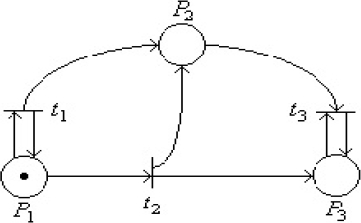
The reachability tree of the Petri net, starting from the initial marking (1, 0, 0) is shown in >Fig 4.

Fig. 4 Reachability tree 

This Petri net model has three paths along its reachability tree, one stable and two unstable. Therefore the discrete event time algorithm results to be partially stable. The ASM program of the discrete event time algorithm that models it, turns out to be composed by the following three ASM programs:

— if   True   then   ϕn1:=(1,n,0),

— if   True   then   ϕn2:=(0,n,1),

— if   True   then   ϕn3:=(0,0,1).

The set of updates is given by Δυ(X)={(ϕn1:=(1,n,0)),(ϕn2:=(0,n,1)),(ϕn3:=(0,0,1))}.

7 Conclusions

This paper introduces the axiomatization, computabilty and stability issues of discrete event time algorithms. Its main contribution consists in proposing a formalization free of any interpretation of discrete event time algorithms and continues discussing computability and stability issues. A Church type thesis, its proof and the notion of stabilty for discrete event time algorithms is proposed. The stability analysis presentation starts concentrating in discrete event time algorithms i.e., discrete event time dynamical systems, whose Petri net model is described by difference equations, and continues considering Lyapunov energy functions in terms of the logical structures of the vocabulary. A stability analysis based on the reachability tree of the Petri net model is also discussed.