


 nueva página del texto (beta)
 Inglés (pdf)
 Artículo en XML
 Referencias del artículo
 Enviar artículo por email
 Citado por SciELO
  Similares en
SciELO
Similares en
SciELO 
 Permalink
1 Introduction
Nowadays, productivity is the major objective for the industrial world to keep competitive in an even-increasing market. So, increasing the productivity can be realized through increasing the availability of the production capacity. To improve the performance of the parks of the electrical energy, it is essential to develop methods and evaluation tools of the residual reliability of the materials to optimize from a technico-economic point of view, the investments of maintenance to be realized. The major difficulty in establishing the Probability laws for the occurrence of components’ failures in the hydraulic system is that” each equipment should be considered as a prototype”, with specificities which limit the relevance of the only use of the statistical approach based on the hypothesis of similar data.
One possible way to overcome this obstacle would be to aggregate the knowledge of different but complementary natures in terms of information on the equipment, by statistical techniques and physical approaches based on models or digital codes characterizing the behavior of the equipment. The statistical approach would make it possible to efficiently identify an ”average generic” reliability law that will be representative of all the components, a law that would then be individualized to each material thanks to the results of the calculations resulting from the physical approach and The historical useful life of each component.
This explains the many recent studies, both academic and industrial, on the reliability of the systems and their maintenance optimization. The maintenance concept has gradually emerged. The benefit of this approach is today recognized by the vast majority of industrialists. However, this recognition is still theoretical because of the underlying practical difficulties in the application of this method.
The available knowledge on the reliability of the system is used to organize its maintenance. This approach is known as ‘‘Reliability Centered Maintenance” (RCM) [1], maintenance based on reliability. The goal of this approach is to optimize the parameters of a maintenance strategy by defining the best compromise between the cost of maintenance of the system and its availability. To realize a study of maintenance based on the reliability requires prior modeling the degradation of considered system, which is difficult task when the system becomes complex.
The first step consists in exploiting the REX database and the expert’s knowledge and advices to estimate the parameters of the model of degradation of the chosen system. The model of degradation is then enriched taking into account maintenance operations. Once the system and its maintenance are properly formalized, a utility function is established in order to evaluate a given maintenance strategy according to one or more given criteria. The objective of the RCM approach is then to maximize the utility function by adjusting the parameters of maintenance to realize the best compromise between maintenance costs and availability of the system. A large number of studies have already focused on the modeling of degradation processes and propose a set of tools or methodologies for modeling the degradation of discrete or continuous states systems. Two main modeling classes are generally considered.
The first proposes methods for developing analytical models describing the evolution of degradation [2]. These approaches concern the mechanical community studying the evolution of fatigue defects. The second modeling class relies on stochastic methods. We are interested in the second class. Indeed, this category is decomposed into static stochastic approaches and dynamic stochastic approaches. In fact, the static stochastic modeling aims to define the end of life moments of the system without being really interested in the dynamics of the degradation.
These approaches present a major interest because of their simplicity of implementation. The most used static stochastic models [3] are: the Exponential model, the Weibull model and the Berthoron model. However, these static approaches are not perfectly adapted to model the dynamics of a system and the dynamic stochastic approaches such as: dynamic stochastic processes, Markov Chains (MC) and more generally all Probabilistic Graphical Models (PGM) are preferred. We are interested in the second class. Indeed, this category is decomposed into static stochastic approaches and dynamic stochastic approaches. In fact, the static stochastic modeling aims to define the end of life moments of the system without being really interested in the dynamics of the degradation.
These approaches present a major interest because of their simplicity of implementation. The most used static stochastic models [3] are: the Exponential model, the Weibull model and the Berthoron model. However, these static approaches are not perfectly adapted to model the dynamics of a system and the dynamic stochastic approaches such as: dynamic stochastic processes, Markov Chains (MC) and more generally all Probabilistic Graphical Models (PGM) are preferred. In our study, we are interested in the dynamic stochastic approaches.
The present paper is structured as follows: the next part, introduces the general concepts of dependability analysis, maintenance strategies and the organization of maintenance based on reliability (RCM). The third section deals with a review on stochastic modeling degradation in the case of maintenance based on reliability. The fourth part details our proposed approach. Then, we conclude and present future work prospects.
2 General Concepts
2.1 Dependability
Nowadays, dependability, presented as the science of failure, is omnipresent in all industrial areas. The objective is to respond to regulatory constraints or competitiveness requirements (productivity, profitability...) and security of goods and people [4].
2.1.1 Definition
Zio in [4] defines dependability as: All the capacities of an item which allow it to perform its function at the appropriate time for the intended duration without damage for itself and its environment. The dependability attributes are generally grouped under the acronym RMAS (Reliability: measures continuity of service, Maintainability: is the aptitude for repairs and evolutions, Availability: which is the fact of being ready to use; for a non-repairable system, availability is equivalent to reliability, Safety: which is the absence of catastrophic or critical consequences for the environment.).
2.2 Maintenance Modelling
2.2.1 Definition
Deloux in[5] defines maintenance as: The set of all technical, administrative and management actions during the life cycle of an item, intended to maintain or restore it to a state in which it can perform a required function”. Maintenance has some objectives. On the one hand, it aims to limit the effects of disturbances( industrial installations are disrupted throughout their operation by malfunctions which affect production costs, the quality of products and services, availability, safety and security of persons) in order to achieve the required performance. On the other hand, maintenance aims to increase the availability of the system, reduce main tenance costs, improve security, or increase the quality of production.
2.2.2 Maintenance Methods
Figure 1 shows the different types of maintenance actions of a system generally grouped into two categories [6].
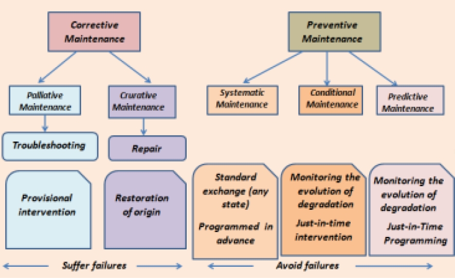
2.2.2.1 Corrective Maintenance
It is the simplest maintenance strategy to implement. It consists in performing a maintenance action whenever a fault occurs on the system. The operations of maintenance are not planned.
According to whether the intervention is final or not, two subcategories of corrective maintenance are defined. The first approach called palliative is provisional. It is often activated in an emergency, when a quick restart of the system is required. In this approach, the system is returned to the operating state as soon as possible without being repaired. The second approach named curative in which the system is refurbished before reboot. In both cases, we wait to undergo the failure of the system and its consequences before taking action.
2.2.2.2 Preventive Maintenance
Unlike the corrective maintenance, preventive maintenance is performed before failure occurs, in order to reduce the risk of failure. The interventions are either programmed in advance according to a timeline, or conditioned by the state of system degradation. The preventive maintenance action can be systematic, conditional, or predictive. The first approach is based on timeline defining the moments (periodic or not) on which the system must be refurbished, whatever its state. The other two approaches require an instrumentation (permanent or punctual) to estimate the state of degradation of the system. Indeed, the conditional maintenance consists in activating maintenance actions conditionally to the current state of the system.
It requires the implementation of a device for monitoring the degradation of the system, called diagnosis. The result of a diagnosis method can be a direct information on the state of the system or information on the Remaining Useful Life (RUL) (case of predictive maintenance).
Indeed, Predictive maintenance consists in activating maintenance actions based on an estimate of the remaining operating time before failure occurs (Remaining Useful Life (RUL). This type of maintenance can be assimilated to conditional maintenance; the difference is that for predictive maintenance it is necessary to extrapolate and predict the evolution of the state of system degradation to predict an intervention. This approach based on prognostics requires a model of degradation of the system. Maintenance strategies are used to define decision rules and determine the information context that determines a maintenance decision space.
2.3 Organization of the Maintenance based on the Reliability
The study of reliability is an essential step both in the conception of a system and in its operational phases. To answer this need, since the end of the 70s, a particular organization of the maintenance was proposed, based on the use of the knowledge that we can have from the reliability of a system. This particular organization of maintenance is known as the RCM. The objective of this approach is to optimize the parameters of a maintenance strategy by defining the best compromise between the maintenance costs of the system and its availability. For a detailed description of this approach, the reader may turn to [1], which gives the first general description of the RCM. This approach follows this organization:
‒ A model of degradation of the system resulting from the exploitation of REX database and/ the expert’s knowledge and advice to estimate the parameters of the model.
‒ A modeling of the maintenance actions and their consequences on the state of the system, based on the existing maintenance repositories (references).
‒ A cost function (utility function) to evaluate a given maintenance strategy from a set of parameters characterizing it.
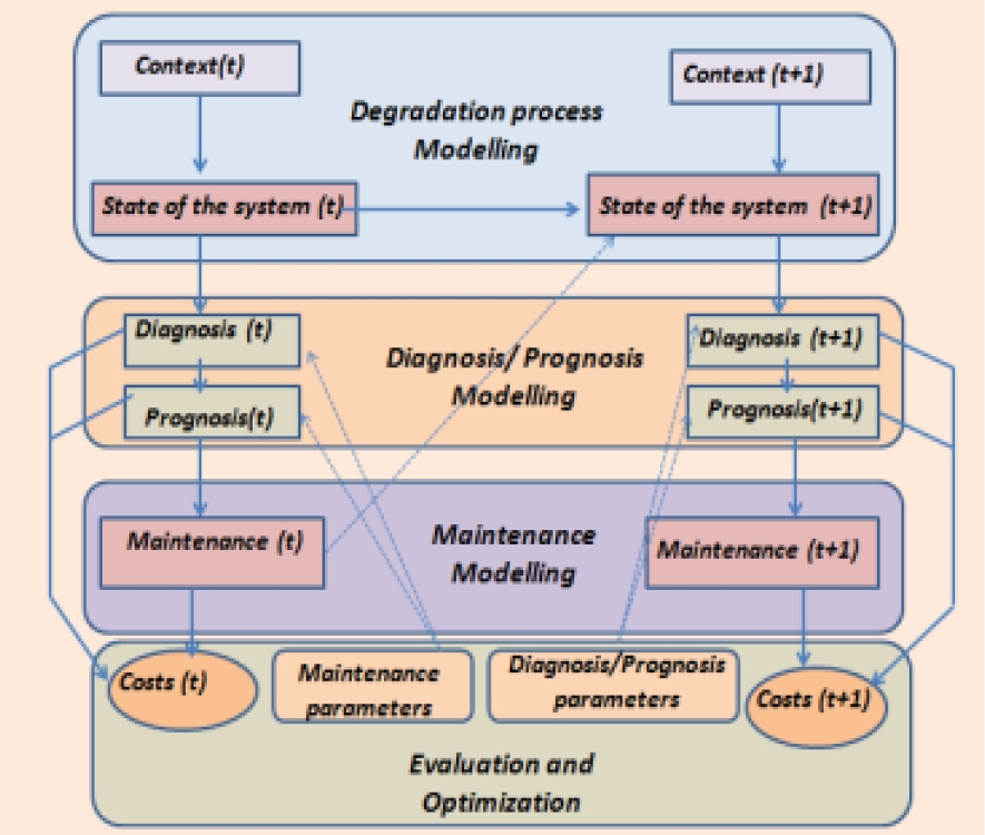
These three models correspond to different blocks of the general architecture to develop models of maintenance. This general architecture is represented in the following paragraph.
2.3.1. General Architecture
A model of maintenance is a set of tools, of models allowing to answer the main questions of the heads of the maintenance department. Such as: is the maintenance policy adapted to their needs, constraints, and objectives? And how to optimize it? These are tools for evaluating, comparing and optimizing the maintenance strategies.
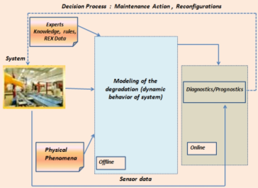
The basis of this architecture [7] is the development of a degradation model to simulate the behavior of the system during its use. This initial phase is the key of any model of maintenance based on the reliability. Indeed, considering an approach based on the reliability, the precision and accuracy of indicators provided by this model will largely depend on the quality of degradation modeling. The next step concerns the modeling of diagnosis and prognosis. Indeed, advanced maintenance strategies integrate monitoring systems that provide information on the state of the system components. These sensors provide information on emerging faults and the generated diagnosis can lead to the release of the maintenance actions.
The “diagnosis modeling” block corresponds to the location of the causes of the anomalies or failures observed on the system. It is based on a thorough knowledge of the system components, the interactions between the components, the operating and environmental conditions and the context in which the system evolves. The “prognosis modeling” block is based on the results of the detection and the diagnosis to predict the duration of operation before the failure of the system. This prediction requires knowledge of the current state of the system and its future conditions of use.
Then, the diagnosis prognosis results influence the maintenance actions related to the estimated state of the system. Maintenance actions modify the system state (or components on which these actions are performed).
Finally, the last module considered for the development of a model of maintenance consists of a set of utilities (cost, gain) associated with the different blocks of the model. Indeed, this model lists the parameters on which the optimization algorithms will evaluate and compare different configurations of maintenance strategies.
As shown in figure 2, the main input of the diagnostic / prognostic process is the state of the system characterized by the degradation model. So we are interested, in the rest of this paper, in the modeling of the degradation process. Indeed, it is essential to build the most possible faithful models of the system behavior and degradation. To do this, it is necessary to choose the modeling tools with care. The modeling must allow translating the involved physical phenomena, to represent the interactions between the system components, to take into account the used data, and the available ways of calculations.
2.3.2. Optimization of Maintenance: Diagnosis vs. Prognosis
The optimization of maintenance is to ensure a certain level of availability of the equipments of the system at a lower cost. In order to avoid the costs due to the breakdown of the system, it is better to anticipate potential failures of the system to avoid them. Indeed, an action of maintenance consists in replacing the equipments of the system, which break down and are not capable to perform their function.
The decision of a maintenance action is very complex and requires monitoring and intelligent analysis of the state of the system.
It must be reduced to the operations of replacing the equipment, which has actually failed.
Longer the maintenance phase, the more expensive it is. Therefore, the necessity for diagnostic methods to detect more exactly the signs of a potential failure in the system and identify the causes of failures in terms of equipments to be repaired. Thus, the diagnosis when performed with efficiency, improves productivity. Based on the information supplied by the methods of diagnosis, prognostic methods can estimate and predict the effects of these failures on the other equipments of the system. Prognostic methods are also used to improve the planning and scheduling of maintenance activities. In order to understand better the field of diagnosis and prognosis, figure 3 illustrates the chronology of the progression of the failure of a system’s component.
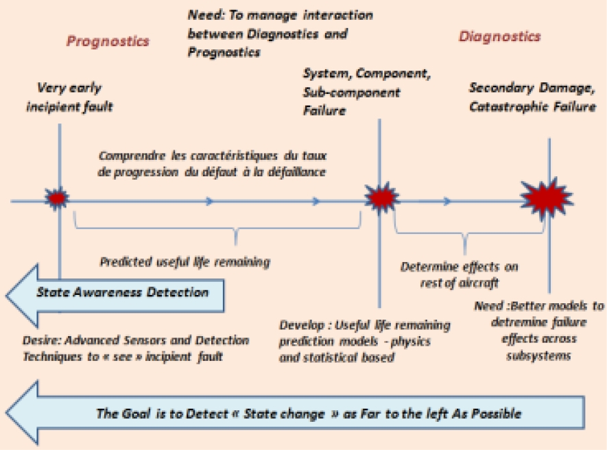
At the beginning of the service life of the component, it is considered as being in good condition. After a certain time of operation, a state of incipient fault develops. Therefore, the severity of default increases until the component finally fails. If the system is allowed to continue operating, it is likely that other damage may be caused to other secondary components or systems.
According to [8, 9], the field of application of the diagnosis generally takes place at the time of the failure of the component, or on the interval between the failure of the component and the possible failure of the whole system. However, if a condition of defect can be detected in an early stage, actions of maintenance can be delayed until the defect progresses in a more advanced state, but always before the failure. At this interval between the detection of an incipient fault condition and the occurrence of a failure, the prognostic domain appears. A sufficient interval between fault detection and system failure allows a range of operational functions and corrective maintenance work that can be planned in advance, with the necessary resources and personnel. In the next section, we present a review of the literature on the various modeling tools used in modeling the degradation process.
3 A Review on Dynamic Stochastic Modeling of the Degradation Process
The main characteristics to be modeled in a degradation process model for assessing reliability and maintenance aspects for dynamic system are: the complexity and the size of the system [10], the nature of multi-state components [11], uncertainties on the parameter estimation [10], the dependence between events such as failure [12], the temporal aspects [13], the integration of qualitative information with quantitative knowledge on different abstraction levels [14].
For modeling these requirements, many works are available and they are divided into two categories [9]. The first category is that of the models with continuous degradation, whereas the second category defines the models with space of finite states (also called multi-state model).
3.1 Continuous Time Degradation Models
In the case of a representation of a degradation process by a continuous model, the state of the system can be determined by a numerical value at each instant. In general, the evolution of the degradation is represented by a series of increasing values (Zt), (Zt >= 0).
Thus, the states of the system are the results on the stochastic realizations on a process with increasing monotonous trajectories. For a relevant estimate, it is necessary to know the law of increasing degradation between two consecutive instants in order to estimate the level of degradation at any time [15]. According to [16], degradation is assumed to be a Markov process. The degradation at a given instant t depends only on the level of degradation at the precedent instant t-t and the time interval between the two instants. This is justified if the only information available on the state of the system is the increase in the degradation of the system between these two instants [17]. The class of Levy processes, which are stochastic processes with stationary and independent increases, is particularly well adapted to the modeling of continuous degradation of systems to estimate and optimize their maintenance strategy. Indeed, Levy processes include processes widely used in literature such as Gamma processes [18], the Poisson processes [19], and the deterministic Markov processes [20].
Among the many authors using Levy processes to model degradation, for example [21] was the first to propose using a Gamma process to model a random failure literature such as Gamma processes [18], the Poisson processes [19], and the deterministic Markov processes [20]. Among the many authors using Levy processes to model degradation, for example [21] was the first to propose using a Gamma process to model a random failure.
In [18], the author proposes a more recent application of Gamma processes for maintenance. In addition, Gamma processes have been used for the prevention of track geometry defects (railway applications) [22, 23]. In [24], the authors also use two different non-homogeneous Poisson processes for the arrival of repairable and non-repairable failures. Based on this model, preventive maintenance is established. In [25], the author considers that degradation follows a stochastic jump-type process. The occurrences of the jumps form a homogeneous or inhomogeneous Poisson process. Moreover, the authors suppose that the time of failure obeys a probability law, which is a function of the level of current degradation of the system and therefore is not defined by a threshold.
3.2 Discrete Time Degradation Models
Discrete time dynamic system refers to a set of each components, which may be in a state, which evolves as a function of a parameter t introducing a notion of order. The parameter t may for example represent a discrete time, a position. [3].
In fact, the dynamic term does not concern the structure of the system, which remains unchanged, but rather reflects changes in the states of the system components over time. The discrete and finite qualifiers reflect the fact that the state space is a countable and a finite set. Figure 4 gives an example of a three-state dynamic system evolution over a discrete time.
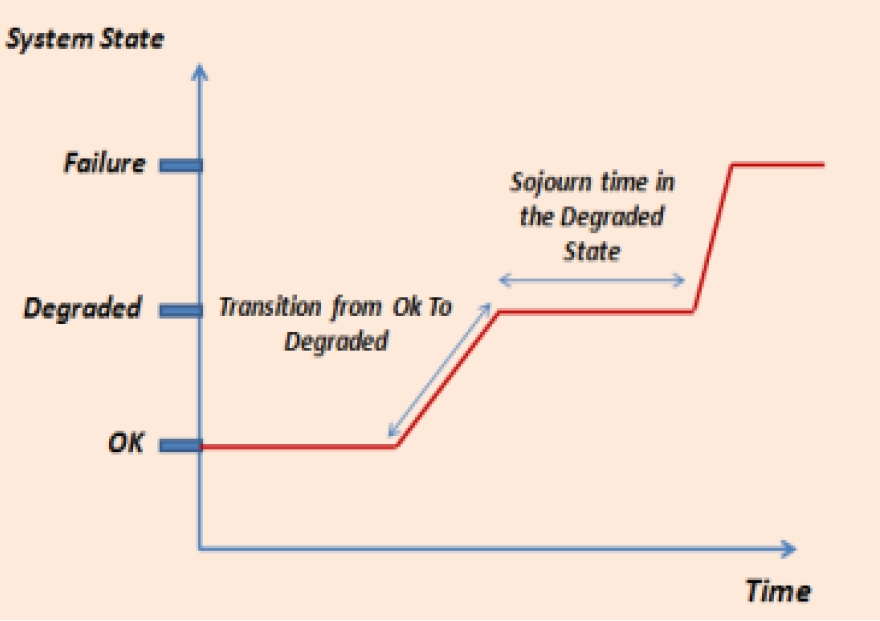
The aim is to model a multi-state system and therefore to capture how the system state changes over time. Indeed, a good modeling of the degradation process must take into account, at best, all the information contained in the observed trajectories of the system (transitions and sojourn time in each state).
Several dynamic stochastic approaches grouped in the family of Probabilistic Graphical Models (PGM) and dealing with reliability analysis constitute tools allowing representing stochastic transitions between different states of a system and they are consequently adapted for the discrete modeling of degradation.
PGMs include Stochastic Petri nets [26], which are powerful tools for modeling, analyzing and evaluating discrete event systems. They form a natural graphical support, which is a precious help for the analysis, and have analytical properties, which allow a simple evaluation of the behavior of the studied system.
Several works on maintenance policy evaluation studies are based on the stochastic Petri nets formalism and associated with the Monte Carlo simulation [27, 28, 29].
The main drawback of using this type of tool is the need for high-performance simulation tools, which are generally very expensive.
Hence, Markov Chains (MC) method is suitable for reliability studies of systems [30]. Indeed, the Markov Chains method allows representing stochastic transitions between different states of a multi-state and multi-component system and the integration of diverse kinds of knowledge. Therefore, the MC is well suited for the discrete modeling of degradation. In [31], the authors use the MC for the dynamic modeling of the degradation, in the aim to deduct estimations indicators of reliability and the lifetime. The authors, in [32], use the MC to model the degradation of the geometry of a ballasted path. In addition, the work of [33] uses the MC to model the evolution of the rigidity of a bridge supporting a ballasted path.
However, the use of MC has many drawbacks. In order to explain behavior and causalities, the modeling of the degradation process becomes more complex with a large number of variables. This requirement constitutes the first drawback. The next shortcoming of this approach comes from the constraint on state sojourn times which are necessarily exponentially (geometrically) distributed. Indeed, this Markovian hypothesis places the system directly into the maturity phase (zone 2 of the “Bathtub Curve” [5]) with constant failure rates. If some systems verify this hypothesis, several industrial applications behaviors are distant from geometric laws. In [7], the authors show that the MC approximation introduces a non-negligible bias in the modeling of system degradation. Therefore, an adapting model of maintenance with to such hypothesis can lead to very significant errors in the estimation of the optimal parameters of the maintenance.
To overcome these limitations, on the one hand, semi-Markov models [34] were developed which allow considering any kind of sojourn time distributions. These tools provide powerful analytical tools when the studied system has reasonable size. On the other hand, the Cox model or a more general proportional hazard model [35] offers an interesting modeling tool when analyzing the effects of the contextual variables on the system degradation. These approaches have the advantage of flexibility on their conditions of use (discrete/continuous time, discrete /continuous variables). However, these approaches are difficult to apply to large systems with a large number of variables.
Moreover, recent works on reliability involving the use of PGMs, based on the Bayesian Networks (BNs) formalism, have been relevant in the context of complex system [36]. In [37], the RBs are used to analyze the reasons for the collapse of the railway bridge.
Then, the authors in [38] explain how to model crossing dysfunction with RBs. PGMs, in particular RBs, allow the modeling of fault trees [39], while the dynamics version called Dynamic Bayesian Networks (DBNs) allows to model Markov Chains influenced by exogenous variables. In [40], the authors explain how to exploit DBNs to model the dynamic degradation system by a Markov Chain. Indeed, the factorization possibility of a Markov model by a DBN permits to reduce the model complexity and to model more complex system. In [41], the authors investigate the use of DBN for modeling the causal relationships between Degradation / cause / consequence.
Then, utility nodes are integrated into the probabilistic problem. However, the analysis of reliability by PGMs in particular by RBDs is not without problems. Indeed, on the one hand, this type of modeling imposes to work in finite and discrete spaces of time and states. To overcome this drawback and avoid the discrete time modeling hypothesis, the Marko jump models [42] have been proposed. In [43], the authors explain how to deal to develop Bayesian Network in continuous time. However, the complexity of the learning and inference algorithms of these networks make it even more difficult to use them for complex applications and are mainly limited to academic works.
The same way, in [44], the authors built hybrid BN including discrete and continuous nodes to estimate the system reliability. The time sampling of the continuous variables is updated by taking account the evidence. Indeed, the authors present this concept as an alternative method to simulation methods such as Markov Chain Monte Carlo (MCMC). On the other hand, the main shortcoming of this approach comes from the constraint on state sojourn times which are necessarily exponentially (geometrically) distributed.
In order to overcome these restrictions, a specific dynamic graphical model called Graphical Duration Model (GDM) based on the RBD formalism, has been proposed [45].
This approach aims to represent complex stochastic degradation process with any kind of state sojourn time distributions.
In [46], the author proposes to use PGMs with an approach based on an engineering approach, ie a system modelling step precedes the transition to a simulation tool. The authors in [47] propose another approach based on PGMs. This approach makes it possible to calculate the probability law of each component and to deduce the residual lifetime of the system.
In [48, 49], the authors formalized the inclusion of exogenous variables representing events (maintenance actions, environmental conditions) in a degradation processes by using an Input Output Hidden Markov Model (IO-HMM). Then, the model of this process is integrated in a systems global model formalized by an Object Oriented Dynamic Bayesian Networks (OODBN).
In the same way, other authors use a classical Hidden Markov Model (HMM) such as the Hidden Markov Model (HMM) [50] or Hidden Semi Markov Model (HSMM) [51] to model the unobservable process of degradation and link it to observations of their consequences.
In [52], the authors show that it is possible to model the level of degradation process using a classical HMM and thus help in the organization and evaluation of maintenance.
In [53], the authors propose contributions for modeling the impact of component reliability on the functional levels of systems by Bayesian networks.
Indeed, Bayesian networks present an inference tool with the incorporation of knowledge on the domain. In [54], first, the authors were interested in how DBN can handle epistemic and random uncertainties. Then, they have integrated the dynamic aspect in this modeling of uncertain processes.
The authors in [55] extended DBN to Evidential Networks based on an extended Bayesian inference. Evidential Networks deal with multi-state systems for reliability and performance evaluation. In the next section, we present the proposed approach.
4 Proposed Approach
4.1 General Description
The proposed approach aims to contribute to the following scientific issues:
‒ Modeling of degradation processes in the case of maintenance based on reliability.
‒ Diagnosis of the state of health of a system and the prognosis of performance, degradation and residual lifetime of a system.
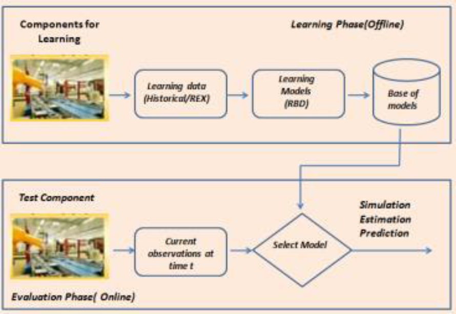
Figure 5 generalizes the modeling approach. Indeed, the use of a dynamic modeling tool allows, on the one hand, to model the causal relationships that exist between the various events and variables of the system and, on the other hand, to take into account the probabilistic and uncertain factor of the values taken by these variables.
This step is performed offline. Then, depending on the models learned in the off-line phase and the current observations of the data available and provided by the sensors, estimates and / or predictions are made online (possibly, off-line through simulation data, for example) to determine the health state and future performance of the system. The results of the diagnostic / prognostic process are used to reduce maintenance costs, improve availability and reliability, and ensure the security of goods and people.
4.2 First Contribution: The Proposed Degradation Process Model
The literature review of classical methods for modeling degradation processes has revealed, to our knowledge, that few approaches allow considering several components having their own degradation mode, while taking into account the influence of context variables on the degradation process and without being limited to a Markov hypothesis.
In fact, there are few methods that incorporate in the modeling of the degradation, on the one hand, the influence factors (such as service time, age, number of requests, and environmental conditions, etc.), the degradation symptoms, the relation between the degradation observation and the appearance of their failure modes, the effects of maintenance activities and the planning and execution of maintenance actions. In addition, on the other hand, the characterization, representation and propagation uncertainties in maintenance studies based on reliability.
In the aim to cover the propagation uncertainties aspect the idea consists in extending the models of the classical HMM family to the Dynamic Probabilistic Graphic Models based on the DBN formalism to allow the modeling of the degradation and its impact on the performance of the systems.
Thus, a temporal propagation of the uncertainty in the form of probability intervals is established in order to solve the problems of diagnosis and prognosis. It is in this context that the learning and inference algorithms are extended. The choice of the DBN formalism is justified by some properties related to the DBN. Indeed, in the first place, the DBN allows a reduction in the number of computing operations by using the new efficient inference algorithms.
This allows realizing a learning of the degradation model and a faster inference in the case of complex phenomena involving several states and / or observation matrices. Secondly, DBN facilitates the representation of complex models by modeling in two layers defining the initial model parameters and the dynamic (stochastic) aspect. In addition, the major difference between an HMM and a DBN is that, in the first model, the state space is described by a single random variable Xt, whereas, for a DBN the hidden state can be represented by a group of random variables X1,..., XNk.
Thus, DBN makes it easier to manage complex systems or variables having dependencies that are difficult to represent by HMMs. On the other hand, the main drawback of standard HMMs lies in the use only of the geometric distribution in the modeling of its duration distribution. Thus, the HMM modeled under the DBN formalism and with integration explicitly the notion of duration in its distribution model. In this way, the obtained HMM can directly model any kind of distribution and consequently offers a significant advantage when used in many applications.
Then, in the objective to cover the influence factors such as service time, environmental conditions, number of requests and the effects of maintenance activities and the planning execution on the degradation process model, a collection of context variables can be used to model the system context. So, the proposed approach is based on modeling tool having the following characteristics:
‒ A typical HHM model represented by the DBN formalism.
‒ The explicit integration of any kind of state sojourn time distribution.
‒ The integration of a collection of context variables (co-variates).
4.2.1 Detailed Description of the Degradation Process Model
The procedure for modeling the degradation of the system and predicting its progression over time is summarized as shown in Figure 6 and described as follows:
-
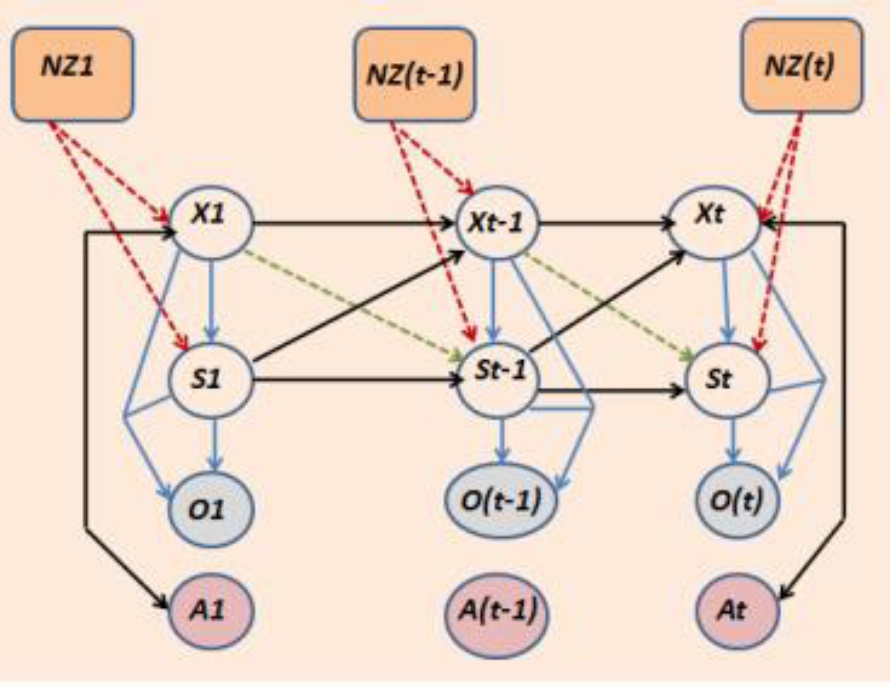
1) Define the variables of the HMM model represented by a RBD (number of states corresponding to the different states of degradation, number of observations corresponding to the characteristics used, duration of stays in different states, context variables (covariates)). Thus the objective is to manipulate the set of (Xt, St, NZt, At) where:
‒ Xt,(1 ≤ t ≤ T ): it is a random variable with values in X, representing the system state at time t over a sequence of length T. It depends on the previous system state X(t−1), the previous remaining duration S(t−1), on contextual variables NZy and on the maintenance activities At. the dependence with X(t−1) defines the dependencies between time slice (transitions from one state to another when arriving at the end of sojourn time). While the dependence with S(t−1) allows to activate the change of state.
‒ St,(1≤ t ≤T ): it is a random variable with values in S, representing the remaining time before a system state modification (remaining sojourn time). It depends on the previous duration variable S(t−1) for the decrementation of the sojourn time and on the current state Xt for the rest of sojourn time when a transition has taken place at time t-1 and, optionally, on the previous state X(t−1) and some contextual variables NZt.
‒ NZt : it is a secondary network representing the influence of context variables on the degradation model whose objective is to define the distribution of a possible collection of context variables (covariates) Zt=(Z(p,t))1≤p≤P that works on variable state Xt and duration variable St.
‒ At, (1 ≤ t ≤ T ): it is a random variable with value in A, representing the maintenance action selected at time t over a sequence of length T and their effects on the degradation model.
2) Representation of the HMM (in this case, we choose the factorial HMM with two hidden nodes X and S and 1 observed node O) model by an RBD (elaboration of the structure and representation of dependencies between time slices and variables) (Figure 7).
3) Learning phase (Off-line): The training data, which are delivered by the installed sensors to monitor the system, representing the degradation history. The characteristics, presented in each historical at the t time, are used to estimate the parameters of the models obtained as well as their temporal parameters (sojourn time in each state). These parameters, which represent system degradation, are obtained through a well-adapted learning Expectation Maximization (EM) algorithm of Baum-Welch, generalized to the DBNs.
4) Exploitation phase (On-line): after the estimation of the parameters of these models, they can be used On-line on new observations to know the health state of the system using the (exact or approximate) inferences algorithms. To do this, the characteristics extracted from monitoring system are conditionally injected into the learned models in order to select the one that represents the best current observation. The selection process is based on the calculation of the probabilities of the different models in relation with the current observation. Thus, the selected model is then used to detect, diagnose the current state of the system and estimate the future performance of system.
4.3 Second Contribution: Towards the Identification of New Features of Prognosis
The objectives of prognosis are to anticipate the occurrence of a phenomenon, which has just occurred and thus allows the operator to avoid the consequence failures, to increase the availability of the system, to improve their security and to reduce the costs of maintenance.
Because prognostic algorithms based on degradation follow the tendency of some measure of degradation, called a prognostic feature, the identification of an appropriate prognostic feature is essential for the performance of the prognostic model. In fact, a good prognostic feature must well capture the trend of the fault progression through the system’s entire lifetime. It is difficult to make an accurate prediction if the trend of the health indicator is not evident throughout the entire life cycle of the system or if the trend is shown just before a failure occurs.
Thus, the scientific issue concerns obtaining the characteristic and monotonic indicators which allow, on the one hand, to detect the first signs of degradation and on the other hand to predict with early enough the failures of the system. Several feature selection methods have been developed. At first, the identification of the prognostic characteristics is left to the analysis and judgments of the experts. Prognostic feature are usually chosen by a visual inspection of the available data which is time consuming and expensive.
Then, many approaches using Artificial Intelligence approaches have been developed [56, 57, 58]. In [59], the authors develop two new defect characteristics called TALAF and THIKAT, which combined with classical characteristics, in the aim to improve diagnosis up to the point where the ultimate signs of catastrophic failures are observed and to diagnose the severity of the degradation of the ball bearings. It is also possible to merge several characteristics into a single health indicator, which is then used to predict the performance using an automated approach, which results in an optimal or near-optimal feature.
As automated approach [60] proposed a method based on the genetic algorithm to identify an optimal set of prognostic features from a population of characteristics and also proposed a set of fitness measures (prognostic suitability metrics) namely, monotonicity, prognosability, and trendability to evaluate the goodness of the identified feature. These measures can be used with any traditional optimization algorithm to identify the appropriate prognostic feature.
The authors in [57] propose to use a metric based on the separability: measure of consecutive time segments in order to evaluate the quality of the extracted feature from the raw signals for the prediction.
An approach based on Genetic Programming (GP) has also been proposed by [61] to identify advanced features with a strong correlation to the defect progression in order to achieve better prediction.
However, it is very difficult to determine a failure threshold of the identified feature especially when different features are involved in the GP. Therefore, keeping the original feature is crucial to determining this threshold failure.
4.3.1 Problem Statement and Description Approach
In a situation where fault-to-failure data is rare and the development of degradation models proves difficult, the problem is whether it is possible to make a good prediction in the absence of prognostic characteristics, which can be identified to represent the fault progression.
We have focused on the identification of new prognostic features possessing the above mentioned qualities. The approach of the proposed prognosis methodology is described in Figure 8.
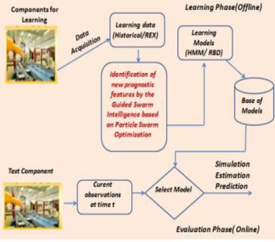
Indeed, we propose a Guided Swarm Intelligence advanced extraction technique based on Particle Swarm Optimization (PSO) Meta-heuristic to reveal the correlation between the prognostic features and the degradation of the system using the set of metrics proposed in [60] and the proposed model in the first contribution (HMM model represented by an RBD and integrating the distribution of the sojourn time durations) as a prognostic algorithm for the prediction of future system performances.
5 Conclusion
In this paper, firstly, the general concepts of dependability analysis, maintenance strategies and the organization of the RCM have been presented. Then, a bibliographical review has been presented on stochastic modeling degradation in the case of maintenance based on reliability. Next, we have detailed our proposed approach, which is based on two contributions.
On the one hand, we have proposed a degradation process model based on tools having the following characteristics: a typical HHM model represented by the DBN formalism, the explicit integration of any kind of state sojourn time distribution and the integration of a collection of context variables (covariates).
On the other hand, we have addressed an identification of new features of prognosis. Finally, in the future work, we will address an implementation and a simulation of the proposed approach.

