


 nueva página del texto (beta)
 Inglés (pdf)
 Artículo en XML
 Referencias del artículo
 Enviar artículo por email
 Citado por SciELO
  Similares en
SciELO
Similares en
SciELO 
 Permalink
1 Introduction
Technological advances strongly depend on the selection and use of specific materials, for example, the uses of steel in the first and second industrial revolution and the role of silicon in electronic applications.
The study of suitable materials for the development of new technology has triggered the uprising of fields such as materials science and engineering, whose goal is to gather basic knowledge of the materials internal structure, the relationship between their properties and the design and applications [6]. Today this science pays special attention to nanomaterials, such as nanotubes. This paper focuses on these structures, particularly in vertically aligned nanotubes (VANT).
There are different techniques for studying VANT, among these it is found the microscopy. It uses optical, scanning electron (SEM) and atomic force microscopes to make these structures visible, see Fig. 1. Image acquisition of VANT is carried out by digital cameras connected to microscopes that have increased their quality and reduced costs in recent years.

In addition, with the development of increasingly powerful computers, a great interest in image analysis for automatic extraction of quantitative characteristics, e.g., to count nanotubes in an image, calculate their size and describe its shape, as come to scene.
VANT characterization is traditionally performed by semiautomatic routines that work on images in the computer, which brings certain disadvantages. Counting these structures manually is a laborious, boring and slow activity, which limits the number of images that can be analyzed. Additionally, measurement of other characteristics, e.g., their diameter may be not representative because only a fraction of nanotubes is considered for calculation.
Finally, since the image characterization is performed by human observers, the process is exposed to subjectivity and might have variability in the measurements when is performed by different people or even by the same specialist.
Automatic image analysis has the potential to overcome the disadvantages mentioned above. First, it is performed using computer resources, which reduces the time and effort required for VANT characterization. Second, it does not require observer’s intervention; therefore the subjectivity problem is overcome because the same parameters and algorithms are used in each image. And thirdly, it can help create versatile tools to work on images acquired by any microscope, not like specialized programs that currently exist.
The aim of this paper is to review recent methods in the image analysis field applied to the automatic characterization of VANT, and serve as a basis for researchers in the developing of computer systems in this specific domain. The methods have been divided into four classes: SEM image restoration, nanotubes segmentation, feature extraction and validation.
2 Nanotubes
First Nanotubes experiments can be trace back to 1952 with carbon nanotubes.
Nowadays, nanotubes are made of a variety of elements and its uses are promising in remarkable fields such as health science and electronic industry, to name a few.
2.1 Definition and Properties
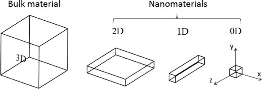
A nanotube is an element of 1D nanomaterial, category in which nanowires and nanofibers belong. Nanomaterials are classified as 3D, 2D, 1D and 0D; it means how many dimensions are above 100 nm (Fig. 2).
Nanotubes can be modified in many ways, associating a foreign element by physical and chemical techniques; resulting nanotubes are called meta-nanotubes. Five different types of association are listed below [15].
Doped nanotubes: nanotubes are associated with electron donor or acceptor elements.
Functionalized nanotubes: where various individual chemical functions are grafted.
Decorated (Coated) nanotubes: the foreign component is a genuine phase, from the point of view of chemistry and structure.
Filled nanotubes: the inner cavity is fully or partially filled with foreign atoms, molecules, or compounds.
Heterogeneous nanotubes: carbon nanotubes whose carbon atoms from the hexagonal graphene lattice are partially or even totally substituted with hetero-atoms.
2.2 Applications
The exceptional electrical, chemical, and mechanical properties made carbon nanotubes (CNT) used widely in the construction of chemical sensors and biosensors, especially in the field of supporting materials [24]. Inorganic nanotubes (especially metal sulfides or oxides) are mostly fabricated to exploit other material-specific properties, and the focus of interest is on biomedical, photochemical, electrical and environmental applications [21,25].
2.3 TiO2 Nanotubes
In materials science, TiO2 nanotubes are one of the most studied compounds because of their wide potential use in photocatalysis, dye-sensitized solar cells, and biomedical devices; reason why they were chosen for this work. These 1D nanoestructures provide highly stable unique electronic properties, such as high electron mobility or quantum confinememnt effects, a very high specific surface area, and even show a very high mechanical strength.
Self-organized oxide tube arrays or pore arrays can be obtained by an anodization process of a suitable metal. When metals are exposed to a sufficiently anodic voltage in an electrochemical configuration, an oxidation reaction will be initiated. The first self-organized anodic oxides on titanium were reported for anodization in chromic acid electrolytes containing hydrofluoric acid by [33]. This work showed that organized nanotube layers (although the author called the structure porous) of up to about 500 nm in thickness. The tube structure was not highly organized and the tubes showed considerable sidewall in homogeneity [22].
3 Scanning Electron Microscope
Since the scanning electron microscope (SEM) was commercialized, material characterization by SEM has shown a remarkable progress. Now, many types of SEMs are being used, and their performance and capabilities are greatly different from each other. Their general use is to obtain high magnification images of conductive or semiconducting samples from different fields of sciences and industry areas. However, implementation of new technological advances allows to obtain images from non-conductive materials, and also the posibility to use the SEM as both, characterization and fabrication technique.
3.1 Working Principles
To be able to use a SEM, it is essential to recognize their features, as well as to understand the reasons for the contrast of SEM images. The scanning electron microscope is used for observation of specimen surfaces. When the specimen is irradiated with a fine electron beam (called an electron probe), secondary electrons are emitted from the specimen surface. Topography of the surfaces can be observed by two-dimensional scanning of the electron probe over the surface and acquisition of an image from the detected secondary electrons [12]. To form the electron probe, the SEM requires basically an electron gun, a condenser lens, and an objective lens. Other components are necessary to, but it could vary because of design, and applications.
3.2 Electron Matter Interactions
Since the interaction electron matter release different types of electrons and signals (see Fig. 3), there are different types of electron and signal detectors for image acquisition in materials science, some of the most commonly used in SEM are the SE (secondary electron), BSE (backscattered electron), in-beam SE, and the EDX detector.

There are two main issues involved in image acquisition, the material composition and the information we want to obtain. For example, non-conductive materials limit the quality of image because of the material charging and the low signal, and the selected signal detector depends on the electron emitted from the sample, secondary electrons are sensitive to the morphology and give information near to the surface, while the back-scattered electrons comes deeper from the sample and give information of the atomic mass. Other photonic signals are emitted from the sample, for example, characteristic x-rays and continuum bremsstrahlung, the x-rays are used to know qualitative elemental composition of the sample.
3.3 Image Processing Mechanism
All the electronic or photonic signals resulting of the electron matter interaction can be used to produce an image according to the detector mechanisms, but the most common is the SE image. The called “raster image” begins in the scan of the specimen by means of a very thin electron beam (a few nanometers of diameter) controlled by electrostatic lens, the magnification depends on the scanned area and the screen resolution, smaller scanned area achieves larger magnification. Once the secondary electrons are emitted from the specimen, a grid whit a low positive voltage attract them, and then are accelerated to reaches the scintillator with enough energy to emit photons, a photomultiplier amplify the signal, the brightness of the image depends on how many electrons reaches the detector and the contrast can be modifying changing the photomultiplier voltage.
3.4 Nanotubes SEM Characterization
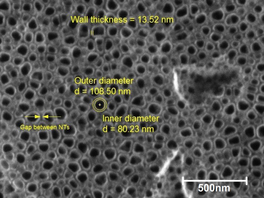
In nanotubes characterization, is necessary to define general properties as the chemical composition, random or aligned growth orientation. Specific features are obtained in individual nanotubes as the length, inner and external diameter, wall thickness, gap between nanotubes, and crystalline structure are the most commonly used fixtures to define the nanotubes (see Fig. 4) [11,28,32].
Above mentioned features are normally obtained by means of several characterization technics; FESEM (field emission scanning electron microscopy), XRD (x-ray diffraction), TEM (transmission electron microscopy), EDX (energy dispersive x-ray spectroscopy), PL (photoluminescence), BET (Brunauer-Emmet-Teller) and XPS (x-ray photoelectron spectroscopy) are the most used [27,29].
In SEM, when a specimen is well known, extract sample features becomes easier. However, this rarely happens and the task begins to be tough. Each analyzed sample has its own image processing issues, but in general, get the optimum contrast and focus is critical to precisely define the edges. Edges are very important in feature measurements. In NT, it is all about edges, since a well-defined edge allows to measure distances, diameters, heights, etc.
In nanoscale, at very high magnification, SEM measurements are very susceptible to electromagnetic and mechanical noise, to avoid this, scan speed is increased and image quality is decreased, losing sharpness and getting inaccurate measurements. Also, acquirable statistics, as average diameter or density, may be a tedious, tired and very slow task, and are susceptible to the issues treated above.
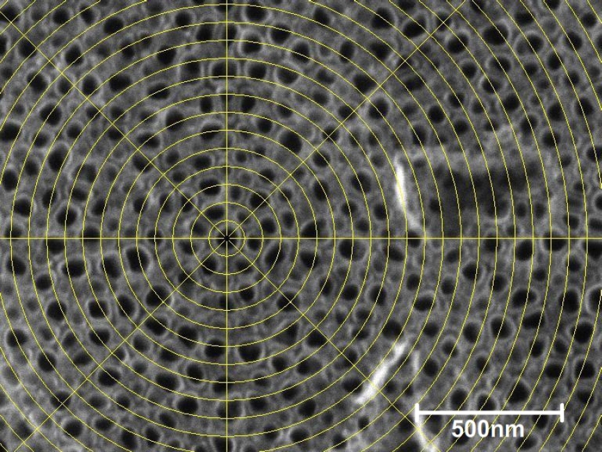
However, depending on the tools at hand, strategies to separate by reduced areas, and manual counting could be used (see Fig. 5).
Actually, SEM’s software offers a wide variety of tools which could be useful in general applications areas, however, the mentioned tools have low performance in specific areas due to its not specialized development.
To overcome this problematic, it is necessary to buy an specialized expensive software or perform a post-processing image analysis procedure.
4 Image Analysis
Image analysis process for the characterization of VANT involves useful information extraction from SEM image database by means of automatic methods (see Fig. 6). According to literature, in order to achieve this, a series of main stages could be followed as SEM image restoration, nanotubes segmentation, feature extraction, validation and data analysis. Some of these are described in detail below. A good example of image analysis to characterize nanotubes can be seen in [2].

4.1 SEM Image Restoration
The main objective of restoration techniques is to recover a SEM image of VANT that has been degraded. To achieve this, it is necessary to know the degradation phenomenon that produced this result.
The principal sources of degradation in SEM images are generated during the acquisition process which is affected by a variety of factors such as: external influences, the fluctuation of temperature in the room and mechanical vibrations; equipment quality, defects and malfunctions of the sensing elements; and operation, the operator’s lack of experience and improper specimen preparation. The factors above listed are attributed to the followings types of image disturbances: noises, blurring, poor quality, low contrast, among others.
Practically, restoration techniques attempt to model the degradation and apply the inverse process, to recover an original SEM image of VANT with good quality. According to [3] this restoration process can be modeled as in Fig. 7, an input SEM image f(x, y) is modified by a degradation function H and additive noise η(x, y) to produce a degraded SEM image g(x, y). With some knowledge about the degradation function and the additive noise, a restoration filter is created and applied on the degraded SEM image to get an approximation

There are exist two types of SEM image restoration techniques, some work in spatial domain and others in frequency domain.
The first operate directly on SEM image pixels and are applicable when degradation is additive noise produced by random processes in the microscope, and the others on the SEM image’s Fourier transform and are chosen to work with degradations such as SEM image blur due to lack of resolution. Below are some of these techniques as long as results generated on degraded SEM images of VANT. For spatial domain, statistic filters and adaptive filters are presented; and for frequency domain, inverse filtering and Wiener filtering.
4.1.1 Linear Filtering
These filters transform a pixel value of noisy SEM image given some neighboring pixels values. This transformation is carry out by statistical operations such as mean, median and mode filtering. In the case of mean filtering, the technique is applied directly in spatial domain that given a noisy SEM image g(x, y) obtains a filtered SEM image
where Sxy is the set of coordinates in a neighborhood of size mxn, centered at point (x, y). For others filters, the pixel values of filtered SEM image are calculated by obtaining the median and mode of noisy image neighborhoods. The following example serves to explain this concept. It has a SEM image region with pixel values 1 and 2, and there is a noise pixel 8 (see Fig. 8). When applying a mode filtering, the noise pixel is transformed to a more representative value of its neighborhood, in this case is 1 because it is more frequently. In [31] an example of the use of median filtering to remove SEM image noise is presented.

In plain words, statistic filters are actually a SEM image smoothing to mitigate or eliminate pixels with very different values in image’s homogeneous regions such as noise and borders. In the case of noise, the desired effect is the elimination of this in the SEM image; and in the case of borders, the result is an attenuation of them [19].
4.1.2 Adaptive Filters
While statistic filters work on SEM images regardless of the change of characteristics and noise from one region to another, adaptive filters modify their operation according to statistical information of the filtering region (neighborhood). For this reason adaptive filters have better performance than statistic filters, greater computational cost and complexity [17]. It is important to remember that these are applied only when the SEM image degradation is additive noise.
Adaptive filters are based on two simple parameters of the SEM image, mean and variance. These measures have a strong relationship with the SEM image appearance, on the one hand the mean represents the average pixel value or intensity in a determined SEM image region, and on the other hand the variance a measure of contrast in that region.
Desired operation of the adaptive filters is to transform a noisy SEM image g(x, y) into a filtered SEM image
where
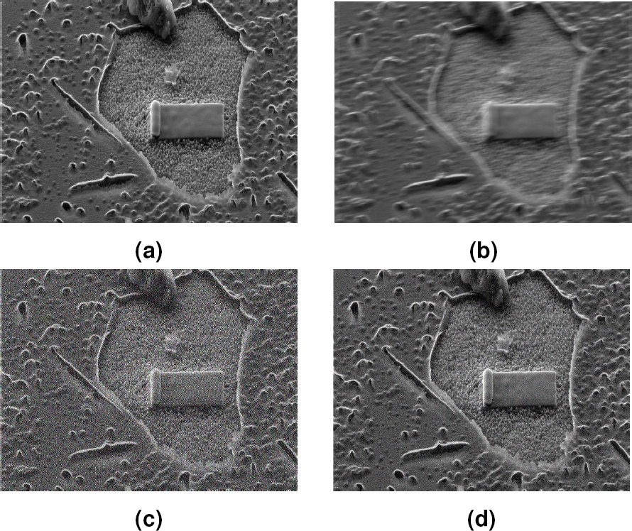
A comparison between a statistic filter and an adaptive filter is seen in Fig. 9. Filters were applied to a SEM image of vertically aligned TiO2 nanotubes with simulated noise. Results (Fig. 9c and Fig. 9d) clearly show that the adaptive filter has a better performance to reduce noise and improve the edges of nanotubes, and therefore it gets a good approximation of the original SEM image.
4.1.3 Inverse Filtering
As already mentioned, a degraded SEM image is the result of modifying an original SEM image by a degradation function and additive noise. The filters seen above, namely, statistic filters and adaptive filters work on degraded SEM images only by additive noise.
Contrary to these, inverse filtering tries to restore corrupted SEM images mainly considering the degradation function and not the noise, reason for which it doesn’t have a good performance in noisy SEM images [23].
Inverse filtering works in frequency domain so it operates on the SEM image’s Fourier transform. Basically its definition arises from the following equation for a degraded SEM image:
where if the noise N(u, v) is despised, it can be obtained an approximation of the original SEM image transform
There is a problem with this definition since a ratio is computed. If the degradation function has zero or very small values, an error may occur in the process and affect the filtered SEM image. One way for avoiding this problem is to assign small values for the filter when this tends to diverge.
Inverse filtering has the advantage of requiring only the degradation function, which can be experimentally determined.
Finally, it is recommended to use this filter on blurred SEM images with very little noise for improving their edges and sharp details, in the presence of noise is better a Wiener filter.
4.1.4 Wiener Filtering
Unlike inverse filtering, Wiener filtering takes into account both the degradation function and statistical information of the noise when trying to restore a degraded SEM image. It reduces the additive noise and inverts the blurring simultaneously. The main idea of the filter is to find a filtered SEM image
In addition to the above minimum error criterion, it is assumed that the degradation function and noise are uncorrelated and that the filtered SEM image has a linear relationship with the degraded SEM image. According to these assumptions and others, it can be found the following expression for Wiener filtering in the frequency domain:
where
A drawback of this filter is the prior knowledge of the original SEM image power spectrum which in practice isn’t available. Moreover, its main advantage is perform well in the noise presence. In [14] a study about carbon nanotubes characterization is presented which uses the Wiener filtering to reduce noise in images and improve their quality.
Fig. 10 shows the results of applying the inverse and Wiener filtering on a simulated blur image of vertically aligned TiO2 nanotubes with Pt protective layer. Remember that this disturbance can be originated by lack of resolution and misconfiguration of the SEM. As can be seen, Wiener filtering (Fig. 10d) obtained a better result than inverse filtering (Fig. 10c) in the image restoration because it reduced noise and clearly defined edges.
4.2 Nanotubes Segmentation
Once the SEM image of VANT is restored, the next step in image analysis is nanotubes segmentation, which aims to divide the SEM image into its interest objects (nanotubes) and background. This is the most difficult and important step because an effective feature extraction method is required. For example, in the characterization of VANT images it’s very common to perform counts and measure diameters and lengths, these features can be extracted easily if the nanotubes segmentation is accurate, otherwise this data may be false. In other words, the correct VANT characterization is strictly dependent on the accuracy of SEM image segmentation.
There are several nanotubes segmentation methods but most are based on two SEM image properties: similarity and discontinuity. The former divides the SEM image into similar regions according to the pixel intensity values; and the later searches for abrupt changes in SEM image intensity (image edges) and uses these discontinuities to assess different regions [18]. This section focuses on the similarity based methods because in the image analysis area applied to VANT characterization are the most used, some of these methods are: thresholding, region growing, region splitting and merging and k-means clustering.
4.2.1 Thresholding
Thresholding is a nanotubes segmentation method widely used for its simplicity and low computational cost whose main idea is to partition a SEM image as follows: Assume a SEM image in grayscale f(x, y) with intensity values distributed into two groups, those associated to the nanotubes and background. To separate them it is possible to choose a threshold value T, so that if a pixel in the SEM image f(x, y) ] T, it is classified as a nanotube pixel, otherwise the pixel is classified as a background pixel. This idea is used in [7] for the automatic binarization of carbon nanotubes images. The above is the case for a SEM image with light objects on a dark background and can be represented by:
where g(x, y) is the binary segmented SEM image, f(x, y) the SEM image in grayscale and T the threshold value. The thresholding can be global, in which the threshold value is calculated once for the entire SEM image; or local, where different threshold values are computed to segment the SEM image based on statistical information of local regions. It is often preferable to use local thresholding because the global is not enough for acceptable nanotubes segmentation because of the noise and nonuniform illumination in the SEM image [1].
4.2.2 Region Growing
Region growing finds SEM image regions directly contrary to the thresholding method, its basic approach is as follows: first, a set of seed points are assigned in different positions of the SEM image to be partitioned, these points initially represent the SEM image regions. Then, the neighboring pixels of each seed are compared against their seed point using a similarity criterion (range of intensity or color); next, if a neighboring pixel satisfies the similarity criterion, it is added to the region represented by its seed point, else it is rejected. After that, a stopping rule is checked to stop regions growth when no more pixels for inclusion. Finally, the procedure is repeated to grow the new SEM image regions and thus achieve nanotubes segmentation [3]:
A similarity criterion used in practice is shown in (8), where fs(x, y) is a seed point in the SEM image to be partitioned, N8(fs) one of the eight neighboring pixels of the seed and T a specified threshold. Some advantages of this technique are the good segmentation results in SEM images with clear edges and its performance against noise. Moreover, it has the disadvantages of over-segmentation due to variation of intensity and its computation is time-consuming [9].
4.2.3 Region Splitting and Merging
Similar to region growing method, it starts with an entire SEM image and divides it into more homogeneous regions. This splitting alone affects the shape of regions and doesn’t produce a good nanotubes segmentation. To solve this problem, it is necessary to perform a merging phase after the splitting. According to [8], the region splitting and merging algorithm is as follows:
Let R represent the entire SEM image or initial region. Select a predicate P (similarity criterion).
If the predicate P is false for any region Ri, split it into four smaller quadrants.
Merge any adjacent regions Rj and Rk that are similar enough.
Repeat steps (2) and (3) successively until no more splitting or merging is possible.
Some advantages of region splitting and merging are: it has a better performance than other nanotubes segmentation methods, allows to select between automatic and interactive techniques to partition an SEM image and is flexible when selecting the segmentation resolution and the similarity criterion. However, this method has the disadvantage that the formulation of stopping rule for nanotubes segmentation is a tedious task and the computation time increases with high segmentation resolution [10].
4.2.4 K-means Clustering
The nanotubes segmentation stage can be seen as a classification process of pixels in two or more classes, foreground and background in the simplest case. This organization of pixels into clusters is known as clustering and it is based on intensity similarity. The well known k-means clustering algorithm is given below [10]:
Determine the number of desired clusters K and randomly assign to each cluster a pixel intensity from the SEM image as its center ck.
Group every pixel to the cluster whose center is closest. The closest normally mean the intensity value is similar.
Recompute the cluster centers. The cluster center is obtained by averaging the intensity values of the pixels belonging to the cluster:
4. Repeat step 2 and 3 until no reassignment of pixels or a convergence criterion is met as certain number of iterations.
The algorithm implementation is easy and it has a lower computational cost compared with other clustering methods. K-means is also flexible because it allows to use one or more pixel features unlike other methods such as thresholding that only focus on the intensity, generally it gives a better nanotubes segmentation.
Some drawbacks of the algorithm is that the clusters number is fixed and the sensitivity of the result depends on the random assignment of the clusters’ initial centers. A use of the k-means clustering algorithm to segment images of nanoparticles is found in [16].
4.2.5 Experimental Results of Segmentation Methods
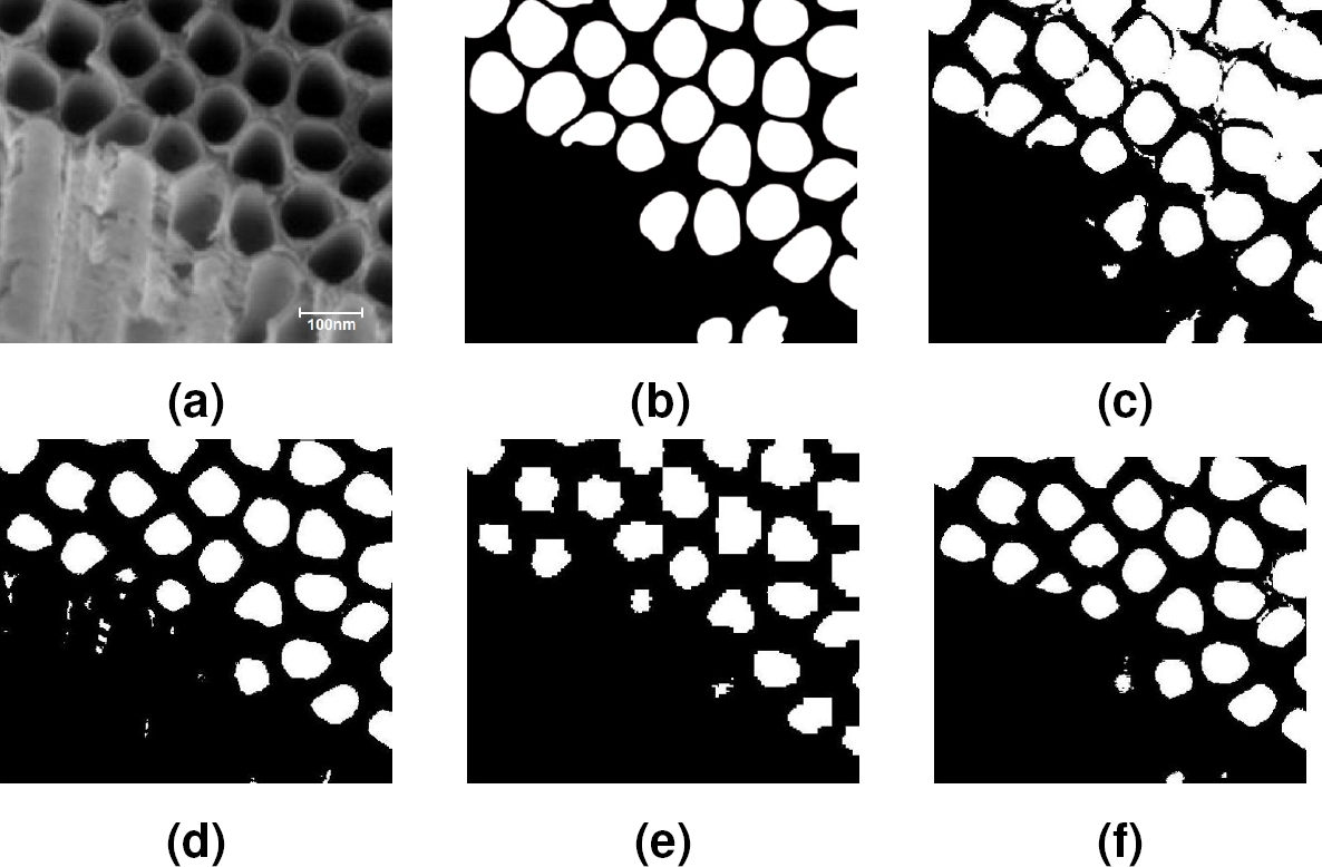
The different segmentation methods were tested on an image of a cross section of TiO2 nanotubes, see Fig. 11. A comparison of these against the ground truth (Fig. 11b) show that k-means clustering achieved the best segmentation result because it has well defined objects (nanotubes are not merged) and a low rate of false positives (background’s pixels labeled as object’s pixels).
4.3 Feature Extraction
At this stage, the features of the detected objects in the previous segmentation are extracted. In our case the objects are nanotubes, thus the features of interest could be: counts, areas, diameters, lengths, density, among others.
Counting nanotubes and their geometric features are simple features extracted directly from the pixels labeling; others such as density (nanotubes number per square unit) and diameter are derived features because are calculated from simple features. Finally there are also higher level features like type of nanotube that require further processing. Some of the methods proposed in literature for calculating these features are presented.
4.3.1 Nanotubes Counting
In order to extract this feature it is necessary the connected components labeling in the binary image of segmentation. The labeling groups the object pixels in components based on pixel connectivity (similar intensity). So all the pixels that belong to the same connected component have equal label, while the pixels that belong to others components get different labels. Generally the labels used are integer numbers, being zero the label for background pixels.
For more information, see [26] for a complete description of the algorithm. Fig. 12 shows experimental results of this method.
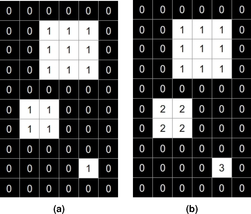
Fig. 12 Connected components labeling. (a) Binary image with three objects and (b) result of the labeling algorithm
As described above, counting nanotubes can be performed as follows: select an original image of nanotubes as that of Fig. 11a, execute some segmentation method to obtain a binary image as shown in Fig. 11b, apply a labeling algorithm to this binary image and get the number of labels corresponding to the total number of nanotubes, which in this example would be 30. Performing automatic counts on images with hundreds or thousands of nanotubes is an advantage of image analysis compared to manual methods because reduce effort and time.
4.3.2 Inner Area
Regarding the area, it can be extracted individually for each object (nanotube) or jointly for all the objects in the labeled image. In the first case, are counted only pixels with a determined label; and in the second case, all pixels except those with zero label. Calculate the area in this way gives a measure in terms of pixels Ap that must be converted to derived units such as square nanometers or micrometers. To achieve this, it is necessary to divide this area in pixels by the number of pixels per square unit N, namely:
where N can be obtained from the information provided at the bottom of a SEM image, in which there is a scale bar showing the relationship between unit length and pixels for that image. With this method it is possible to simultaneously obtain the area of a large number of nanotubes in the image, thus achieving a more representative measurement of this feature and others.
4.3.3 Diameter and Density
As mentioned, diameter and density are examples of derived features, which means they can be obtained from measurements of simple features such as counts and area. One of the most used methods to measure the diameter of a nanotube with irregular shape is to assign it to the diameter of a circle with the same area. This procedure allows to use the formula:
where d is the diameter of a nanotube and A its area.
Others equivalent diameters of a nanotube commonly used in practice are Martin’s diameter and Feret’s diameter [5]. On the other hand, if density is defined as the number of nanotubes per square unit, either square nanometer or micrometer, this can be calculated dividing the counting nanotubes in a region of interest C by the area in square units of that region A, in other words:
Density is a feature useful for characterization of nanotube forests. Finally, remember that these two features (diameter and density) can also be extracted globally in images as Fig. 4, bringing the advantages mentioned above.
4.3.4 Gap between Nanotubes
This feature refers to the average distance between nanotubes in an image. For its measurement it is necessary to get for each nanotube the distances with its N neighboring nanotubes. According to the literature the choice of ”N” is regularly 6, but also can be made based on the visual perception of the image and choose a higher or lower number. Next, an algorithm for obtaining this feature is presented [4]:
Get the centroid coordinates (x, y) of each nanotube.
Fit on each nanotube a circle of radius r with center (x, y).
Calculate the distance between two nanotubes as:
4. Store the N distances of each nanotube with its neighnors.
5. Calculate the average gap between nanotubes.
The algorithm implementation has the advantage of automatically providing an average measure of the gap between all nanotubes in an image without the need to calculate it individually as in Fig. 4.
A disadvantage is that the algorithm can perform an imprecise estimation of the distances when the nanotubes are too close.
4.4 Validation
After the nanotube’s features have been extracted, the next and last step in image analysis is to validate that these are correct. To perform this, it is necessary to have an images dataset whose correct features are well known and compare them against the results obtained by the image analysis methods. In literature, the images dataset is known as ground truth and it is assambled mainly in two ways, by manual inspection of samples under microscope or by computer and using simulated images [18].
In the first way, a group of experts select a set of samples (e.g., nanotubes) and characterizes them either directly under microscope or by using semiautomatic computer programs on their digital images. It is recommended to repeat this manual characterization several times for reducing effects such as the subjectivity of experts on the results [30]. In the second way, the ground truth is obtained by simulation software that generates images based on parameters specified. For example, it could simulate an image whose number of nanotubes and areas are known. Here there is not subjectivity problem because the images are always created with the same algorithms; however, these may not be sufficiently similar to real experimental images.
After obtaining the ground truth data, the following is to use its images as input of the image analysis system and to compare the correct characteristics with those obtained by the feature extraction procedures. If there is similarity between both characterizations, it is said that implementations of the methods perform satisfactory; on the contrary, the methods that provided incorrect measurements of the features must be implemented again, and this is based on an error tolerance defined by experts. Finally, it is recommended to test the system with real images which could represent cases that will be found later and with important challenges such as noise, blurring and lighting changes.
This effectively to ensure robustness and good performance of the system.
4.5 Characterization of VANT
Next it is presented an example of automatic characterization of VANT by image analysis. Two images of vertically aligned TiO2 nanotubes were used and the following methodology was applied to these: for the image restoration stage an adaptive median filtering was performed, the segmentation was carried out by the k-means clustering algorithm, and finally the feature extraction was made with the formulas mentioned above.
Fig. 13 shows the segmentation results over the two images to visualize the nanotubes detected and Table 1 presents the characterization results of the two images with the applied methodology. The extracted features were: number of nanotubes (count), average diameter and area, gap between nanotubes (GBN) and density. The results obtained are presented in the column approximation while the correct results in the column ground truth.
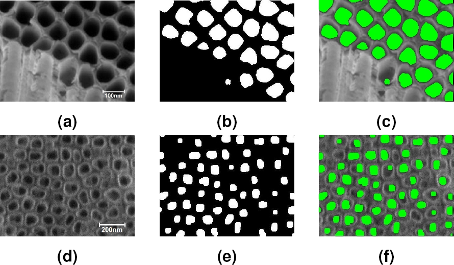
Fig. 13 Nanotubes detection. Segmentation results over two images to visualize the nanotubes detected
Table 1 Characterization results of the two images with the applied methodology
| Image in Fig. 13a | ||
| Feature extracted | Approximation | Ground Truth |
| Count | 29 NTs | 28 NTs |
| Diameter | 70.28 nm | 70.08 nm |
| GBN | 27.95 nm | 28.25 nm |
| Area | 3879.30 nm2 | 3857.26 nm2 |
| Density | 90.62 NTs/µm2 | 87.50 NTs/µm2 |
| Image in Fig. 13d | ||
| Feature extracted | Approximation | Ground Truth |
| Count | 61 NTs | 69 NTs |
| Diameter | 90.70 nm | 115.91 nm |
| GBN | 21.79 nm | 18.81 nm |
| Area | 6461.08 nm2 | 10551.94 nm2 |
| Density | 32.44 NTs/µm2 | 36.70 NTs/µm2 |
As can be seen in Table 1, the approximation obtained for the image in Fig. 13a was acceptable compared against the ground truth. This result is due to the good quality of the image, the small noise and high contrast allowed a good image segmentation (see Fig. 13b) that was crucial for the posterior feature extraction. In the case of the image in Fig. 13d which has a poor quality, it was not achieved a good approximation of features. Here, the nanotubes detection (61 NTs of 69 NTs) and the diameter measurement (90.70 nm against 115.91 nm) were affected by the lack of contrast and noise.
This example shows that the methodology applied produces acceptable characterization results on good quality images, but not in the opposite case. Some recommendations to improve these results are include image contrast techniques and morphological operations for a better detection of nanotubes.
A similar example is found in [20], where an image analysis system for properties assessment of VANT is presented. It is provided a novel way of a surface bioactivation in titanium dental implants. The system is based on advanced image processing and includes restoration, segmentation and classification methods. It works with images of vertically aligned TiO2 nanotubes obtained with SEM and extracts the following essential parameters for the nanomaterial characterization: inner tube area, tube wall thickness and residual space between tubes.
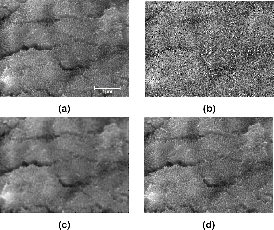
Fig. 14 shows the detection results of the parameters mentioned above with the presented system. Because of the image quality, the system does not detect all nanotubes, but a representative set is obtained to evaluate mean values of the parameters as shown in Table 2.

Fig. 14 Parameters detection. (a) the original image, (b) tube walls detection, (c) non-tube objects detection and (d) all objects detected. Source: [20]
Table 2 Results obtained with the presented system, source: [20]
| Parameter | Sample No. 1 | Sample No. 2 |
| Inner tube area ± std (nm2) | 5372 ± 2164 | 5454 ± 2444 |
| Wall tube thickness ± std (nm) | 33 ± 4 | 36 ± 6 |
| Non-tube objects (%) | 23.1 | 22.4 |
| Non-classified space (%) | 15.7 | 20.2 |
These results are considered significant in the samples assessment but in the paper there is no comparison against the ground truth (correct measurement of parameters). Finally, the system could be applied in nanomaterial quality assessment.
Currently, there are tools for image processing and analysis that can be used to characterize VANT, e.g., ImageJ. The main usage of this software is to calculate particle features as average size, spacing, wall thickness and nearest neighbors; in this case the particles could be tubules or pores located randomly in a sample. A use case of ImageJ is shown in [4], where the measurement of tubule diameter and their spacing in tubular scaffolds is performed. Fig. 15 shows the segmentation and feature extraction results for a SEM image of a tubular scaffold in that paper. As can be seen, this tool provides an automatic way to characterize tubular structures which can be applied easily to vertically aligned nanotubes.

Fig. 15 Tool for image analysis. (a) SEM image of a tubular scaffold, (b) its segmentation after using ImageJ and (c) results table listing some extracted features. Source: [4]
5 Conclusion and Future Work
In this paper the main characterization of SEM issues oriented on the image visual inspection methods used to extract TiO2 NT features were presented. It was established the advantage of using images analysis for characterization over manually methods. Faster performance and objective analysis are properties added to this characterization. Improved images has been obtained by image restoration, overcoming some work conditions, physical limitations, and human factors; as electromagnetic and mechanical noise, equipment resolution and technician lack of expertise, issues that partially or totally limit the capacity features extracting.
The performance of a image analysis system for VANT characterization strongly depends on the segmentation step. The system’s ability to detect nanotubes (interest objects) and background in a SEM image is seriously affected when a degraded image by noise or blurring; in this case, segmentation is inaccurate and therefore the characterization results as well. To avoid this problem, it is recommended to pay special attention in the image restoration and segmentation steps. Comparative studies (quantitative and qualitative) of different methods in each step should be made in order to identify, select and implement the most appropriate for the system.
Image analysis can help to develop versatile systems that work with images taken by different microscopes, which is an area of opportunity because the current professional programs to study and characterize VANT operate only on one type (either SEM or AFM images) and they are expensive hardware. Image analysis can also make possible the correlation of SEM and AFM images to perform topography, composition and 3D studies with a single system, which could even do other tasks such as to simulate the growth of nanotubes.

