1 Introduction

Robot arms are programmable electro-mechanical devices designed to carry out specific tasks such as assembly, material handling, and loading of a tool for: welding, painting, spraying, etc. To understand the complexity of robots, engineering knowledge of design, manufacturing, mechanical, electrical, computer science and mathematics are required.

Applications and developments in the field of robotics have been increasing over time and demand trained graduates who must be proficient in all the technologies related to it.

Teaching engineering courses and specially robotics, is an important subject in undergraduate and graduate school. Engineering educators agree that experience with the real world cannot be taught just in the classroom, hands-on tangible experience is needed.

In addition, it is well known that the more active and pragmatic the students are involved in applying a subject, the better the learning of its theoretical aspects. That is why laboratories are paired to theoretical classes to combine these two important learning aspects. Thus, when teaching a robotics course, it is recommended the use of an experimental platform in the learning process [²] as it allows a practical experience demonstrating the basic concepts and keeping the students' interest and motivation.

A possible platform are commercial industrial manipulator robots, but this constitute limited resources for students to access because of their high costs for institutions. In addition, they could be only used through their proprietary motion description languages, which are specifics to any given manufacturer, requiring to spend long time learning any of them, and the user won’t be involved in designing aspects of the robot. However, even if an industrial robotic design is trying to be built, it is still difficult to achieve, because its parts require long, and expensive processes operated in specialized laboratory equipment to generate an industrial design.

A more reachable platform could be built with open hardware/software philosophy. In this case, the robot designer must deal with concepts like rigid links which are interconnected by joints into a serial chain and manipulated with servo motors in the so-called Joint space. Additionally, there is another Cartesian space where objects and task are defined to operate. Transformation between Joint and Cartesian space and vice versa is the issue of kinematics and it is required for any robot arm.

Hence forward kinematics is defined as transformation from joint space to Cartesian space whereas inverse kinematics is defined as transformation from Cartesian space to joint space. Solution for kinematics is available in algorithms written into specialized libraries. That is the case of the open source Matlab Toolbox for robotics: Robotics Toolbox, this has been translated into a series of different languages such as Python, SciLab and LabView.

The Toolboxes have some important virtues. First, they have been available for a long time and have been used by many people for different problems. So the code could be said to have a high degree of reliability. The Robotics Toolbox [¹] is a software package that allows a MATLAB user to readily create and manipulate datatypes fundamental to robotics such as homogeneous transformations and trajectories. Functions provided, for arbitrary serial-link manipulators, include forward and inverse kinematics.

When considering moving the joints, the driver could be an open-source hardware resource. These has grown up in the last times, offering many possibilities in open platforms, and every time come new products at low cost. Open hardware offers the possibility to educators and researchers to add and program the hardware devices as they want, making the systems completely customizable. In the case of robotics, there is a tendency towards open hardware products [³] because its low cost and easy development.

Thus, the need to develop an experimental platform to serve the purpose of a permanent laboratory for universities and research institutions is justified.

To emphasize on the general principles and provide the student with both a theoretical appreciation of, and practical design and construction experience, a robot arm manipulator has been developed. It is especially valuable for many universities with limited economic resources.

Therefore, it is a good alternative for such robot because it is inexpensive to build.

This paper shows the design, manufacturing, mechanics, electronics, and software of an educational robot arm manipulator. Additionally, mathematical model for the forward and inverse kinematics problems were implemented by the educational robot arm model. A GUI software interface of great importance was developed to use the physical robot arm together with its virtual mirror.

The platform prototype is a robotic arm manipulator with 4 degrees of freedom (DOF). The arm consists of four servomotors: the base, shoulder, elbow, and the wrist, where a marker is hold as a tool. The motor control is performed by a servo controller Arduino UNO that allows a serial connection to send and receive commands to a computer.

The robot arm has been taken as a case study; it utilizes Matlab/Arduino as the tools for testing the characteristics of the robot. The developed platform is used as an educational tool. This work will continue to increase the education, training, research and development possibilities for robotics classes and research in graduate and undergraduate studies.

2 Background

Educational robotic research efforts have been reported in the literature. In [⁴] a robotic course was developed in Korea integrating the use of LEGO kits, humanoids, and industrial robots to improve competitions in engineering education. The author presents an approach to teaching robotics to undergraduate students that used modular, reconfigurable robots developed at LEGO. These kits are accessible in cost, permitting students to acquire experience in the kinematic design of fixed robot manipulators. But students, in fact, did not build the robots.

A commercial 5 DOF robot with the CRS CataLyst-5 from Thermo Fisher Scientific Inc. was controlled through a Matlab/Simulink open-architecture interface, being mostly a software project [⁵]. With [⁶], an educational robotic arm was built, but the interface to it, is through Matlab/Simulink, so the robot can be used just for experimented programmers.

Others educational robotic arm were thought as remote laboratories developing e-learning potentialities in the field of robotics tele laboratories. A virtual training environment was created through a commercial SCARA-type AdeptOne-MV robot arm, a video camera, and an internet connection [⁷].

A tele laboratory was also created to access remotely a SCORBOT ER-V PLUS robot based on Web by using the free open-source software: Scilab, Comedi and Linux [⁸]. In the two previous projects, the students acquired design ability by doing active learning, in a tele laboratory characterized by high immersivity. Virtual laboratories were accessible 24 hours a day and allowed the students to practice their robotics skills at home and at their free time. However, students were focused more on training than in robotic design.

The virtual robotic systems represent an illustrative and cost-effective solution. However, such systems, being mostly soft, may not offer the necessary exposure corresponding to the real robot performance. Virtual models do not address the complexities such as backlash, friction, non-collocation, etc. associated with the physical systems. Typically, the accuracy and credibility of results obtained in a simulated environment are not comparable with physical experiments.

Additionally, training platforms based on commercial robots and development of software had been reported. In [⁹] the GUI software for kinematics of a commercial 5 DOF Lynx-6 was developed. Visual Studio.Net 2005 was used for the implementation. Students learn how to use knowledge and techniques to carry out a set of standard tasks for robots.

A robotic arm was used to test the sliding mode and computed torque control strategies. But no detail on the construction of the robot was given, neither an educational aspect of the project was especially underlined [¹⁰].

BRACON robotic arm based on Dynamixel servomotors and Python software was developed [¹¹]. The project presented a low-cost robotic arm with a nice GUI, but important details of links mechanical design were not shown.

An industrial robotic arm was taken to be modeled using D-H methodology and to generate simulated trajectories based on computer vision techniques [¹²]. In more hands-on approaches, students can develop their own robot structure and then program it with a language. There have been found several papers addressing different areas of teaching and learning with robots for the development of suitable teaching curricula.

A 6 DOF robotic arm was built and reported in [¹³]. Servomotors were used, details of the design were given, a nice GUI was created, but no solution of the inverse kinematic problem was done. A particularly good effort to amplify access to practical experiences in educational robotics was done in [¹⁴]. The activities implemented with this platform included: playing, building, exploring, programming, competing, and learning various science subjects. However, it was completely centered in Lego Mindstorm kits, which is not adequate for university courses and research because of its limited hardware. In addition, no fabrication processes skills were developed in that project.

There are some papers documenting the use of many different low-cost open-source microcontroller cards based on ARM processors. Given that the main purpose of these works was to build a low cost open-source platform to introduce robotics concepts, any card could be suitable since high computational resources were not required. However, its programming should had been simple because maybe the students did not know much about programming or perhaps, they were learning it.

A good review of low-cost open hardware microcontroller boards was given in [¹⁵]. Arduino, Raspberry Pi and BeagleBone among others were mentioned. These boards are useful to control educational platforms like Lego. Arduino support for Simulink software was proposed to control the hardware. In [¹⁶] an ED722C 6-DOF commercial robotic arm was used to be motion controlled through a camera seeing objects in the robot’s workspace.

The project was more interested on the technical aspects of the tasks development instead of getting educational goals. In [¹⁷] Arduino was used to control several types of robots like line followers, bug-like, boat-sailer, explorer and battle oriented.

Arduino arose in 2005 and due to its low cost and open hardware policy, in a few years it has achieved widely spread within the scientific and research community as the brain of various kind of projects.

The Robotics Toolbox [¹] provides a diverse range of functions to simulate arm type robots. The original Toolbox started in 1990 and was dedicated only to arm type robots and supported a very general method of representing the structure of a manipulator with serial joints using objects of Matlab. Arbitrary manipulators with serial links can be created and the Toolbox provides functions for direct and inverse kinematics and dynamics.

The Toolbox includes functions to manipulate and convert between data types such as vectors, homogeneous transformations and unitary quaternies which are necessary to represent position and three-dimensional orientation.

Other Matlab toolbox for teaching, modeling and simulation of robotics manipulators had been developed like [¹⁸]. This toolbox has been called ARTE (A Robotics Toolbox for Education). Another Matlab toolbox had been developed; it is called ROBOLAB and includes into its library the 16 different 6-DOF fundamental serial robot manipulators [¹⁹].

A very convenient GUI allowed the movement of virtual robots chosen in the software. Both toolboxes: ARTE and ROBOLAB, by far, are not so deployed and accepted like the Corke’s one [¹].

3 Design and Construction

Through 3D CAD software for mechanical modeling: SolidWorks, the basic link was created by means of a draw with real measurements. This is done in order to later build and assemble each of them together with its servomotor and, with four of them, form the articulations and links, needed for the construction of the final assembly.

The development of the piece in software allows seeing the characteristics that the element has before manufacturing it, this facilitates finding errors and making the corrections that correspond. Two terminals were designed for each link that contains the assembly until the end-effector.

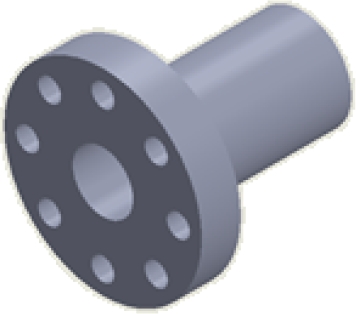
The link (figure 1) that was designed has two terminals, each one on one end and with a different function. The one on the right has a rectangular hole that holds the servomotor to the link with screws.

The one on the left, has the function of connecting with the next link in the kinematic chain. Figure 1 shows the design of the link on an aluminum framework that is the material selected to make the piece.

Fig. 1 Mechanical flat of aluminum framework 

The circular connection, leftmost connection on figure 1 is connected to the next link, through a servo hub, which runs perfectly through a servo block kit. The servo hub is made of aluminum, it has a length of 1”, a hub diameter of 1”, a shaft diameter of 0.5”, and utilize the 0.77” hub pattern (figure 2).

Fig. 2 Servo hub 

The aluminum framework has ends bent at 90°, which allows the piece to function as a reinforcement structure. In addition, the material is light, resistant and easy for machining. There was access to a CNC milling machine DYNA MACH EF8035 to perform the machining by means of chip cutting by turning a 3/8" cutter with 4 cutting edges.

Through milling, it is possible to machine the most diverse materials, such as wood, steel, cast iron, non-ferrous metals, and synthetic materials, on flat or curved surfaces.

The case of aluminum is particularly soft when cut. In addition, the milled pieces were roughened and tuned to avoid roughness. To operate the CNC milling machine, a program in G code was wrote, this is the most used in this type of numerical control machines.

In general terms, G-code is a language by means of which computer-controlled machines and tools can be told what to do and how to do it, for this machine, the 4M software was used. These actions are defined by instructions on where to move, how fast to move and what path to follow. The G codes can be those that contain movements and fixed cycles and M, those that are auxiliary functions. Next, the simulation stage comes, it helps the designer of the piece to foresee and detect problems related to the design before it even physically being built. Hence offering a much more efficient development stage in terms of time and cost.

Figure 3 shows the simulation of the machining of the link at the end of the servomotor. During the process of the simulation, it is possible to observe by which places the cutter is passing and, in this way, some possible error can be found. It is also possible to see in which parts it is, where the milling machine is cutting and in which it is not, this by means of the color of the lines that the simulation leaves. If they are marked lines it is when it is cutting and those that are weaker color is when it is just making a quick movement.

Fig. 3 Rectangular cut simulation 

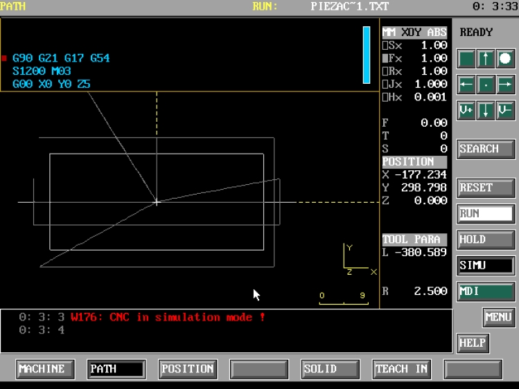
Figure 4 displays the milling of the link at the end of the servomotor. Figure 5 demonstrates the simulation of the milling of the link at its connecting end to the next link. The physical machining of the link is performed at the connection end to the next link, figure 6.

Fig. 4 Machined of link, servo edge 

Fig. 5 Circular cut simulation 

Fig. 6 Machined of link, next link connection edge 

The material that is machined is the 1mm thick aluminum framework with irrelevant measures since the code was designed so that this does not matter. That is, the machining starts only from a center and from there it opens. The proper speed and rotation speed must be specified to obtain adequate machining.

To increase a servo’s load-bearing capabilities is necessary to isolate the lateral load from the servo spline and case. It can be done by using a servo block. The servo block allows users to create complex, extremely rigid, structures with ease using standard Hitec servos. Using a clamping hub on the 1/2” aluminum servo shaft provides an easy way to adjust the position of the component attached to the ServoBlock.

The robust aluminum framework acts as a servo exoskeleton, greatly enhancing the mechanical loads the servo can withstand. The .77” hub pattern is repeated throughout the framework to allow endless attachment options. It is compatible with all standard size Hitec servos. Figure 7 displays a Hitec servo attached to a servo block kit. The robot arm rotational joints are controlled by dedicated servo motors. Servomotors are some kinds of traction elements.

Fig. 7 Servo block kit and servo 

The servo selected was the powerful Hitec HS-625MG. This high-quality servo is perfect for mechatronic and robotics needs. This element is one of the strongest metal gear servos that is available and at a low cost. The HS-625MG servo comes standard with a 3-pin gold plated power and control cable. The HS-625MG can take in 6 volts and deliver 94 oz-in of maximum torque at 0.15 sec/60°.

The servomotors have an acceptable accuracy, given in milliseconds. They can be manipulated by any microcontroller with PWM module, in this case, the Arduino UNO. The microcontroller for example, produces a pulse width, this is sent into a servomotor input, and it can respond with a movement given in degrees.

In this approach being described, four servo motors are controlled to form the kinematics chain. For the robot arm being developed, the base link is the one that most care must be taken, because of the lateral loads it is imposed. A swivel hub connection was used on the base link to allow a 360° horizontally rotation.

The swivel hub lets the connection of any two parts together and has them swivel a full 360°. Internal ball bearings allow for smooth motion. Four holes are on both sides, making attachment easy. Figure 8 shows the swivel hub.

Fig. 8 Swivel hub 

However, the servo motors draw considerable power and must be fed with enough power supply. For this purpose, a 18W 6-in-1 based on the LM350K voltage regulator was built. It provides 6 VDC @ 3A, 18W max output. It takes a 110VAC, 50/60Hz input. Figure 9 illustrate the power supply and Arduino UNO servo controller.

Fig. 9 Power supply & controller 

Servo motors have three wires: power, ground, and signal. The servo’s power wire should be connected to the 6V pin on the power supply. The ground wire should be connected to a ground pin on the power supply and the Arduino board. The signal pin should be connected to a digital pin on the Arduino board. To facilitate these connections special 3-feet long cable was built; it is seen in figure 10.

Fig. 10 Special connection cable 

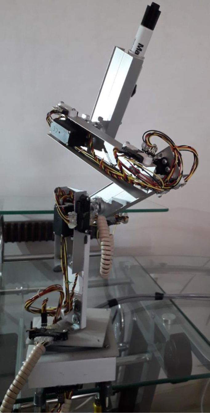
The final mechanical assembly of the prototype of the real robot along with all its wiring and the end-effector, a marker, is revealed in figure 11. This building stage allows students to get acquainted to various aspects of technical design, teamwork, and material constraints. In this stage, design errors frequently occur like building too big links, selection of weak motors, structures stressed because of its own weight or selection of an inappropriate material. These errors had to be overcome to have an operative arm. Figure 12 displays the serial communication scheme between the computer, which is using MATLAB® / Robotics Toolbox [²⁰] and the Arduino; as well as the communication by train of pulses of the Arduino (library Servo) and the servomotor.

Fig. 11 Robot on rest position 

Fig. 12 Robot communication scheme 

A sequence of four consecutive integer values is sent to serial servo controller from the computer. These are a sync byte ($), the desired position joint for each of the four servos (q_i) and the final character (#). Rotational position of each of the servo motors is determined by the specific angle (q_i) by an internal servomotor’s closed loop feedback.

4 Modeling

The kinematics defines the movement of a body as the transformation from its Cartesian space to its joint space and vice versa [²¹].

A manipulator with serial joints contains a chain of joints and mechanical links. Each joint can move the league of its neighbor further away from its nearest neighbor to the origin. One end of the chain, the base, is fixed and the other end is free to move in space, the latter holds the end-effector. The kinematic modeling of a robot is categorized into forward kinematics and inverse kinematics.

The forward kinematic problem consists of determining the location of end-effector in the work space, i.e., position and orientation with respect to a coordinate system that is taken as reference. It is determined based on the joint variables and the parametric values of the robot configuration given by its D-H parameters [²²]. The inverse kinematics problem refers to finding the values of the joint variables that allows the manipulator to reach the given location [²³].

For a manipulator with N joints, numbered from 1 to N numbered. Link 1 is the base of the manipulator and link N loads the end-effector. The joint i connects the link i-1 to the link i and therefore the joint i moves the link i-1. A link is a rigid body that defines the spatial relationship between two neighboring joints. A link is specified by two parameters, its length a_i and its rotation α_i. The joints are also described by two parameters.

The displacement of link d_i is the distance from one joint to the next along the axis of the joint. The angle of the joint θ_i is the rotation of one joint with respect to the next around the axis of the joint. Transformation link matrix is shown in (1):

4.1 D-H Parameters

The structure of articulations for the robot is described by a chain of joints of Revolution. A systematic way of describing the geometry of a chain of serial joints was proposed by Denavit and Hartenberg and is implemented into the Matlab’s Robotics Toolbox [¹].

Next, Table 1 shows the Denavit-Hartenberg parameters for the robot developed. The following segment of code shows variables defining the D-H parameters into the Matlab program:

Table 1 D-H Parameters, angles (Rad), lengths (cm) 

Link	θi	di	ai	αi	offset
1	q1	12	0	-π/2	.222π
2	q2	0	12	π	1.22π
3	q3	0	12	π	1.33π
4	q4	0	0	-π/2	.888π
5	q5	10	0	0	0
6	q6	0	0	0	0

4.2 Forward Kinematics

Forward kinematics is expressed as the pose of the end-effector of the robot arm according to the values of the joints. Homogeneous transformations are used; these are simply the product of the transformation matrices of each individual joint.

A manipulator robot with six articulations or degrees of freedom (DOF) allows reaching an arbitrary pose in the end-effector. The transformation of the manipulator is written as ​60T for the 6-axis robot [²⁴, ²⁵].

The first three columns in the matrices represent the orientation of the end effectors, whereas the last column represents the position of the end effectors.

The forward kinematics problem is concerned with the relationship between the individual joints of the robot manipulator and the position and orientation of the end-effector.

Forward Kinematics equations are generated from the transformation matrixes (4)-(9) and the forward kinematics solution of the arm is the product of these six matrices identified as ​60T.

The approach divides the forward kinematics problem in two parts. From ​10T to ​32T is the elbow manipulator part and from ​43T to ​65T the wrist movement description. Elbow manipulator and wrist are defined through D-H methodology.

The direct model is the relation that allows determining the matrix column x of operational coordinates of the robot corresponding to a given configuration q, see (2):

x=f(q). (2)

The direct geometric model of a robot can be obtained from the homogeneous transformation matrix of the robot that defines the N links of the terminal link with respect to the link 0 of the base of the robot. In the case of simple structure of robots, the transformation matrix is given by (3):

​60T=​10T​21T​32T​43T​54T​65T. (3)

Equations (4-9) are the transformation matrices for each link:

​10T=|Cq10−Sq10Sq10Cq100−10d10001|, (4)

​21T=|Cq2Sq20a2Cq2Sq2−Cq20a2Sq200−100001|, (5)

​32T=|Cq3Sq30a3Cq3Sq3−Cq30a3Sq300−100001|, (6)

​43T=|Cq40−Sq40Sq40Cq400−1000001|, (7)

​54T=|Cq5−Sq500Sq5Cq500001d50001|, (8)

​65T=|Cq6−Sq600Sq6Cq60000100001|. (9)

The code below is the calculation of the forward kinetics made in the project using the Corke’s fkine Toolbox method [¹]:

4.3 Inverse Kinematics

Inverse kinematics is a procedure that seeks to obtain the required joint coordinate values q, given the desired Cartesian pose of the end-effector x. This is a more difficult problem than forward kinematics. On the contrary of forward kinematics, there exist multiple solutions in inverse kinematics [²⁶, ²⁷]. Some constraints can be used to decrease the number of solutions for simplicity. Into Corke’s Robotic Toolbox [¹] there are two methods useful to solve the inverse kinematics problem:

1. Closed-Form solution (algebraic and geometric methods).

2. Numerical solution.

For the first one the kinematics equations that relate the joint variables to the end-effector pose are nonlinear and the Toolbox gives only a restrained description of the manipulator in terms of kinematic parameters. The robot must have 6-axis; also, the robot must have the three wrist axes intersect at a single point (spherical wrist).

For the case of robots, which do not meet this specification, an iterative and numerical slower solution is implemented.

The numerical solution takes advantage of the differential equations that relates joint rates to end-effector velocities, which are linear. It takes the form of (10), which can be easily solved but produces joint rates, rather than the joint values themselves:

V=J(q)q˙, (10)

where q = [q₁, q₂, ..., q_n]^T is the joint variable vector and q˙=[q˙1,q˙2,…q˙n]T is the joint rates vector and produces spatial velocities V = [v_x, v_y, v_x, w_x, w_y, w_z]^T.

In order to track a trajectory that can be described by a sequence of desired pose matrices at regular time intervals t_k along with desired end-effector velocities V(t_k) the joint rate vectors can be computed based on (11).

q˙(tk)=J[q(tk)]−1V(tk). (11)

Using the numerical integration approximation shown in (12) joint variable vector for the next point on the trajectory is calculated.

q(tk+1)=q(tk)+q˙(tk)Δt, (12)

Δt is the time interval between points on the trajectory.

It should be small enough to minimize computation errors from one step to the next on the trajectory. The kinematic inversion, based on the manipulator Jacobian, is applicable to robots of any architecture but requires a nonsingular Jacobian matrix at every point on the trajectory, which is rank deficient compared to the maximum of the Jacobian, singularity is stated in (13).

|J(q)|=0. (13)

At the singularity, joint rates will go to infinity; but even if the robot is close to a singularity, there is the problem for some Cartesian end-effector velocities that require extremely high joint rates.

An alternative for this problem is to use the Jacobian transpose.

The Jacobian transpose transforms a wrench applied at the end-effector to torques and forces experienced at the joints, see (14):

Q=JT(q)g, (14)

where g is a wrench which is a vector in the world coordinate frame of forces and moments.

g=[fx,fy,fz,mx,my,mz].

Q is a joint force vector. The elements of Q are joint torque or force for revolute or prismatic joints, respectively. This mapping from the wrench to joint forces differs from the velocity because singularity will not happen, as it can be for velocity, since the Jacobian’s transpose is used.

This property is harnessed to solve the inverse kinematic problem into the Corke´s Toolbox numerically. The Toolbox develops this approach based on the forward kinematics and the Jacobian transpose which can compute for any manipulator configuration, these functions have no singularities. Into the Toolbox this approach assumes a special spring between the end-effector of the different poses which is pulling and twisting the robot´s end-effector toward the desired pose with a wrench proportional to the difference in pose. The robot has virtually viscous dampers so the joint velocity due to the applied forces will be proportional (15):

q˙(tk+1)=Q(q)/B, (15)

where B is the joint damping coefficient. The update for the joint coordinate is the same as (12).

This algorithm is implemented into the ikine Toolbox method [¹] and is used in this project in the fragment of code below.

There, an incremental pose kinematics inverse is used in order to have world (x, y, z) displacements by using the same Rotation submatrix R_3x3, and varying Translational submatrix T_3x1 into the Homogeneous Transformation matrix:

5 User Graphics Interface

The need for a graphical interface (GUI) is very important because it requires a user-friendly interface for users who have limited programming knowledge.

It is also required that GUI be intuitive, in such a way that anyone familiar with a computer can easily handle the robotic arm just using buttons, text boxes, sliders, etc., and observe changes in both virtual and physical robot arm.

The graphical interface designed for the four degrees of freedom robot (figure 13) was programmed using the MATLAB® software and presents a compact version compared with interfaces developed in other projects, such as [²⁸].

The interface that was created has four controls (buttons: q+, q-, edit box: Deg, and a slide bar) that modify the angle of one of the four joints that is specifically selected to be changed (Joint). It constitutes the direct kinematics. Also, this modification of the angle is changed in one of four intervals given by the selection that is operated in Increment.

Fig. 13 Graphical Interface 

The selection that affects the articulation space (Joint) also affects the World space (inverse kinematics) by selecting one of the three references (wx, wy, wz) for an incremental movement. There is a selection to visualize the virtual robot from four different points of View.

The Home button sends the robot to its resting position. The Store option stores a joint position in memory and increases the Index. The Del button removes the joint position indicated by Index.

The Save button saves all the joint positions of the robot to a *.mat file, thus recording a trajectory. A trajectory is a spatial construction, a location in space that leads from an initial position to a final position. The Load button loads a *.mat file with a path to the robot. The Run button goes through the joint positions that constitute the path to be traveled.

When one of the joint controls is activated, the change produced is observed graphically in the virtual robot. Similarly, the updated value of the joint variable can be seen in the Deg edit box. The position of the slide bar for the modified joint is also updated. Table 2 describes in detail each of the controls of the developed graphical interface.

Table 2 Controls of the interface 

Control	Description
	Select the specified joint to be rotated.
	Select the specified angular or linear increment to be moved.
	Select the specified world frame of reference to be moved.
	Select the specified point of view for the robot.
	Controls that change the angular position of the selected joint.
	Controls that change the selected world frame by a specified increment.
	Sends the robot to Home.
	Motion over all the saved positions.
	Index changes automatically when a position is stored or deleted
	Store a position
	Delete a position
	Save a trajectory to a file
	Load a trajectory from a file

When the virtual robot in the software moves, the same program sends the joint positions (q₁, q₂, q₃, q₄) to the controller (Arduino UNO) through the serial port so that these changes can be seen in the servo motors of the real robot (figure 14).

Fig. 14 Virtual nd real robot arm 

6 Results

After mathematical modeling (D-H) and kinematic solutions were generated and implemented by the software, a Robot arm was developed and tested in this study.

Several trajectories were generated, one of them with the shape of a full circle (figure 15), this was done in order to evaluate the adequate generation of joint positions obtained by solving the direct and inverse kinematics equations by Matlab's Robotics Toolbox.

Fig. 15 Evaluation of generated positions 

7 Discussion

The realization of this project allowed, since the beginning, the enrichment of a senior-level undergraduate robotic course showing many positive results. Students were very enthusiastic because their exposition to a real case of study, also they learn to work in teams in the design and construction of the robot. The students divided tasks among themselves and scheduled their work.

The course was organized in accordance with specific goals. The first goal was to design the robot, CAD was used to design the main mechanical pieces under certain specifications, and such was the case of the robot’s links.

The second goal was to develop manufacturing processes, where the students were challenged by machining pieces with Computer-Aided Manufacturing (CAM) software/machines. In addition, they constructed mechanical and electrical assemblies of the manipulator robot using tools such as band saws, drills, soldering irons, and multimeters.

The third goal was to integrate mechanism, electronic, and computer control, carrying out the achievement of a functional robotic prototype. Here the spectrum of topics required for developing the actual robotic device were components like mechanisms, structures, actuators, drivers, power sources, wiring, microprocessors, peripherals, and real-time programming. Because of the emphasis upon integration, the project centered on laboratory experiences in which student configured, designed, and implemented mechatronic devices.

The fourth goal was the implementation of kinematics. Here concepts were exposed starting from mathematical foundations, such as matrix algebra and trigonometry. Students were introduced to the concepts of direct and inverse kinematics, singularity definition and avoidance, joint rotations, translations, and trajectory computation. Furthermore, in the fifth goal, students demonstrated kinematics concepts developing and programming laboratory experiments with working robotic arm, with the programming environment.

To make the laboratory experience more like real, the six goal was devoted to put the complete experimental robotic system together and to make it move. Students stablished serial communication between computer and microcontroller’s embedded communication library.

Students wrote scrips in Matlab language inserting functional and structural parameters; homogeneous transformations, D-H, calculation of position and orientation of the tool, direction of the joint rotation in the kinematics model, which must coincide with the rotation of the robot’s servo motor. Evaluation the extent of the workspace by varying the joint angles through the reachable space. Scripts should consider joint limitations, and thus joint angles into both, the arm controller and script, must be inside of the physical limits. Therefore, testing of robustness of the code was developed.

Then, the final goal consisted of the script ran in Matlab environment. Students did a final check of the manipulator behavior; they had some specific task to do with the robot. Students programmed the robot to follows a planned path, stored in a *.mat file; as the motion was performed, a draw was painted by a marker on a board.

A static obstacle in the robot path was put, introducing complexity to the task. From that experiment, students understood concepts such as posture (high and low elbow) and its connections with options chosen during the computation of the inverse kinematic. The previous task was repeated, but including a field of obstacles, this had repercussions on the path, precluding the robot from moving into areas previously specified as areas to avoid.

All goals of curriculum were reached, and students took advantage of the robotic course very much. However, existing opportunity areas were identified for further improvement of the robot design.¹

8 Conclusion

The objective was achieved, this is that a low-cost educational and experimental manipulator robot arm of 4 degrees of freedom was designed and built; It took advantage of the most current open hardware and software technology. It can be used in graduate and undergraduate robotic courses to realize didactically the relationships between theoretical and practical aspects of robot manipulator motions in real time. The article described the most relevant details as practical laboratory exercises of the mechanical structure, the electrical and electronic aspects, and the software developed for its management.

Thus, the design of the links was made through SolidWorks. These were machined in a CNC milling machine programmed with G codes. Mechanical exo-skeletal structures were added to reduce the effect of lateral loads on the links. The final assembly was carried out together with the wiring, power supply and controller for the physical robot. The robot was modeled mathematically using the Robotics Toolbox, solving direct and inverse kinematics and an attractive and intuitive GUI interface was created in Matlab.

The controller program was loaded with serial communication and the Servo library of the Arduino. Several tasks (trajectories) were carried out to evaluate the performance of the prototype, resulting in an adequate functioning. All these laboratory exercises provided invaluable hands-on experience that complemented classroom lectures, which are essential for many other aspects of robotics education.

Students showed enthusiasm in the application of the concepts discussed during the lectures, solving the problems by teamwork. In the future, our goal for the robotics educational platform is to integrate formally the prototype with the entire robotics curriculum, increasing the number and type of laboratory exercises routinely conducted by students of robotics track. Therefore, the platform finds its higher potential applications in educational, academic, and research sectors, representing a very encouraging starting point to further development of these activities.