SciELO - Scientific Electronic Library Online

 
vol.24 número3Costo mínimo para trabes rectangulares de concreto reforzado con cartelas parabólicasFuzzy Parameter Adaptation in Genetic Algorithms for the Optimization of Fuzzy Integrators in Modular Neural Networks for Multimodal Biometry índice de autoresíndice de materiabúsqueda de artículos
Home Pagelista alfabética de revistas  

Servicios Personalizados

Revista

Articulo

Indicadores

Links relacionados

  • No hay artículos similaresSimilares en SciELO

Compartir


Computación y Sistemas

versión On-line ISSN 2007-9737versión impresa ISSN 1405-5546

Comp. y Sist. vol.24 no.3 Ciudad de México jul./sep. 2020  Epub 09-Jun-2021

https://doi.org/10.13053/cys-24-3-3326 

Articles

Controlling 2D Artificial Data Mixtures Overlap

Mohammed Ouali1  2  * 

Walid Mahdi1 

Radhwane Gharbaoui3 

Seyyid Ahmed Medjahed3 

11 College of Computers and Information Technology, Taif University, Arabia Saudí, mouali@tu.edu.sa, wmahdi@tu.edu.sa

22 Thales Canada Inc., Canada

33 Université des Sciences et Technologie, Département d’Informatique, Algerie, radouane.gharbaoui@univ-usto.dz, sa.medjahed@univ-usto.dz


Abstract:

Clustering methods are used for identifying groups of similar objects considered as homogenous set. Unfortunately, analytic performance evaluation of clustering methods is a difficult task because of their ad-hoc nature. In this paper, we propose a new test case generator of artificial data for 2 dimensional Gaussian mixtures. The proposed generator has two interesting advantages: the first one is its ability to produce simulated mixture for any number of components, while the second one resides in the fact that it formally quantifies the overlap rate which allows us to add some complexity to the data. Clustering algorithms and validity indices behavior is also analyzed by changing the overlap rate between clusters.

Keywords: Clustering algorithms; unsupervised learning; Gaussian mixture; Gaussian components overlap

1 Introduction

Clustering methods are defined as unsupervised learning processes used to divide a set of observations into clusters [36, 38, 31, 28]. Clusters are groups of similar observations which are sufficiently far from each other. Several clustering methods are defined in the literature and all share a common nature - the difficulty in their analytical evaluation [39, 3, 9, 23, 14].

The discrete frequencies of observations and the measures of similarities between entities and clusters produce many local minima which disturb the process of clustering to converge to the correct results. Therefore, one avenue is to evaluate clustering algorithms using artificially constructed data. Many authors have categorized unsupervised classification based on criteria such as similarity or dissimilarity measures, the nature of data, and the function to be optimized [18]. Based on evaluation, the two principal categories are hierarchical methods and mobile centers methods.

The ultra-metric inequality is one of the most often used methods to generate artificial data to evaluate hierarchical algorithms [10, 22]. A large number of popular methods are based on employing the mixture model and particularly the Gaussian mixtures [15, 2, 25, 26]. The mixture models must satisfy some properties that conform with the clustering methods [24]. These patterns are summarized in two criteria: the internal cohesion and the external isolation.

Internal cohesion ensures observations within the same cluster have similar properties. External isolation ensures observation from different clusters are very dissimilar. Several works in the literature considered the Gaussian distribution as design block for clustering algorithms due its well-known properties [15, 2]. On the other hand, several approaches have been proposed to generate artificial data. Salem and Nandy [30] proposed different structures for producing artificial observations in 2D spaces. The main rule to preserve the internal cohesion of the components mixture is to introduce empty space between the clusters despite the fact that empty space is not a sufficient condition to guarantee external isolation. In the case where the mixture components have close enough centers, no clustering method has the ability to identify the components [30]. In [34, 35], well separated data is generated for 2D and 3D cases.

The two criteria characterizing the cluster structure are strongly respected. Milligan [23] developed an algorithm for generating artificial data but was only able to avoid the total overlap for the first dimension. The claim is that avoiding overlap for the first dimension allows by transitivity to avoid total overlap for the rest of the dimensions [8, 29]. Milligan’s algorithm is verified by visual inspection. Kuiper and Fisher [20] and Bayne et al. [5] directly manipulated a variable which measured certain parameters as separability for a simple covariance matrix of normal clusters. Blashfield [6] and Edelbrock [13] used unconstrained multivariate Gaussian mixture with fairly complex covariance structures.

This allows to obtain cluster structure and the clusters are well separated [14]. Other authors have inserted noise in well separated data to add some complexity to the obtained simulated data [30, 34, 35]. Baudry et al. [4] proposed a verification method to estimate the Gaussian mixture model. This work clearly distinguishes cluster structures of the mixture where the components are well separated from the Gaussian mixtures in case of total overlap. In [17, 37], the authors proposed a new artificial data generator that embeds the notion of the rate of overlap for uncorrelated 2D artificial Gaussian data.

In this paper, we propose a new automatic method for generating artificial data by controlling mixture components overlap. This work tackles two main problems: the design of an artificial data generator for correlated 2D data, and the study of the behavior of clustering algorithms and their respective validity indices by varying the rate of overlap between the mixture components. We are interested in correlated data because of the growing number of applications in computer vision and image processing, as clustering is used as the core solution to solve problems such as segmentation and image matching. In these applications, correlated data that revealed useful when combined and could be used in the clustering process are pixel gray-level, local window gray-level, and local variance.

In this paper, we will show how the overlap rate is quantified and its use as the basis block in the artificial data generator. The rest of this paper is organized as follows: section 2 briefly presents the Gaussian mixture; section 3 deals with components separation; section 4 presents the quantification of component overlap; in section 5, the control of overlap is developed; the generation algorithm and the experimental results are shown in sections 6 and 7 respectively. Finally, the conclusion is drawn with some perspectives.

2 Bivariate Correlated Gaussian Mixture Model

Mixture models are widely used in many applications because many real and natural phenomena as well as sets of data in many disciplines are based on such distributions [14, 1, 3, 25, 30]. A mixture of M Gaussian 2D components is given by:

P(x,y)=j=1MκjGj(x,y,θj),

where j=1Mκj=1 and θi=(μxj,μyj,σxj,σyj,ρj) denotes the parameters of the jth distribution Gj. Gj is given by:

Gj(x,y)=Aexp(12(1ρj2)[t12σxj2+t22σyj22ρjt1t2σxjσyj]),

where A=12πσxjσyj1ρj2, is real and strictly positive. t1=(xμxj) and t2=(yμyj). μxj, μyj are the component center coordinates. σxj and σyj are the standard deviations of the first and second dimension respectively. ρj is the correlation coefficient between the two dimensions X and Y.

3 Well Separated Components

Initially, the clustering methods and the validity indices were evaluated by using well separated data before using any other simulated data. Most works are not based on a formal way to generate artificial data and the main technique to construct isolated mixture components is visual inspection [35, 34, 11, 4].

The objective is to propose a definition that helps qualify and quantify well separated components by involving all the mixture parameters. Mixture components are considered well separated if they exhibit a minimum overlap between clusters [25, 26]; we define:

{xint=μ1+4σ1,xint=μ2+4σ2, (1)

where xint is not really the intersection point, but for a value sufficiently far from the centers of the two components, xint is approximated to be the intersection point. To be more precise in our description, xint is the unique intersection point between C1 and C2 where C1 (respectively C2) is the projection of the intersection point between component Γ1 (respectively Γ2) and the line Δ1:y=κ12πσ1e8(Δ2:y=κ22πσ2e8). But, for xint value sufficiently far from the center of the two components, xint is approximated to take the form of the equation 1. In a Gaussian cluster, 99.7% of the observations belong to the interval ]μ3σ,μ+3σ[, which indicates that the above minimum definition implies the presence of empty spaces between data.

In [17], we presented in 2D the minimum overlap between two components Γ1 and Γ2 so that the intersection point after the projection satisfies:

{Γ1(xint,yint)=κ12πσ1xσ1y1ρ12e8,Γ2(xint,yint)=κ22πσ2xσ2y1ρ22e8. (2)

As in the 1D case, more than 99.7% of the observations are located inside the ellipse defined by the intersection of the plane defined by z1=κ12πσ1xσ1y1ρ12e8 (respectively z2=κ22πσ2xσ2y1ρ22e8) and Γ1 (respectively Γ2), where the condition of minimum overlap for the 2D data guarantees the presence of empty space between the data.

The probability density function of the generated data (pdf ) is constrained to have the same configuration for the well separated components so that:

Definition 1: Two adjacent Gaussian components Γ1(κ1,μx1,μy1,σx1,σy1,ρ1) and Γ2(κ2,μx2,μy2,σx2,σy2,ρ2) are well separated if the intersection point between C1 and C2 is a unique point, where C1 is the projection of the intersection points between Γ1 and the plane T1:z=κ12πσx1σy11ρ12e8, and C2 is the projection of the intersection points between Γ2 and the plane T2:z=κ22πσx2σy21ρ22e8.

Formally, Γ1 and Γ2 are well separated if:

{Γ1(xint,yint)=κ12πσx1σy11ρ12e8,Γ2(xint,yint)=κ22πσx2σy21ρ22e8, (3)

where (xint,yint) is the coordinate of the highest intersection point from among the infinity of intersection points between the two components. Figure 1 shows a mixture of two well separated components.

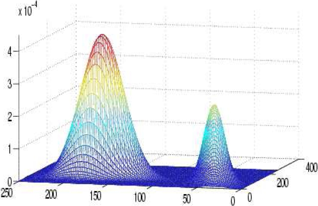
Fig. 1 An example illustrates the minimal overlap between two components of a mixture. Γ1 (0.4, 60, 40, 23, 12, 0.3); Γ2 (0.6, 73.96, 167.98, 10, 20, -0.4) 

3.1 Components Overlap

During the generation of a large set of data, it is important to ensure that the generated mixture components are not in a case of total overlap. Components in a case of total overlap violate the two criteria of internal cohesion and external isolation.

To better explain the meaning of total overlap, let us examine the example of figure 2. In figure 2 (a), the mixture is composed of three components; however, only two are visible; the total overlap can only be detected by visual inspection. A case of maximum overlap is shown in figure 2 (b). We can still distinguish that there are three components. In figure 2 (c), there is a partial overlap between the three components of the mixture. It is clear that the mixture is composed of three components:

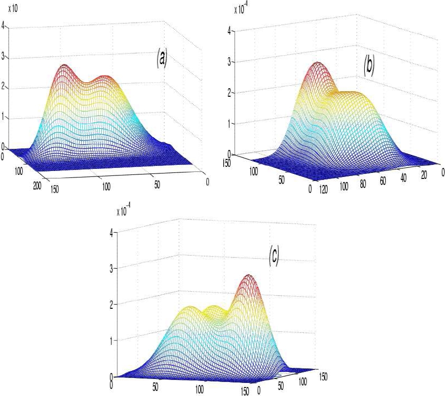
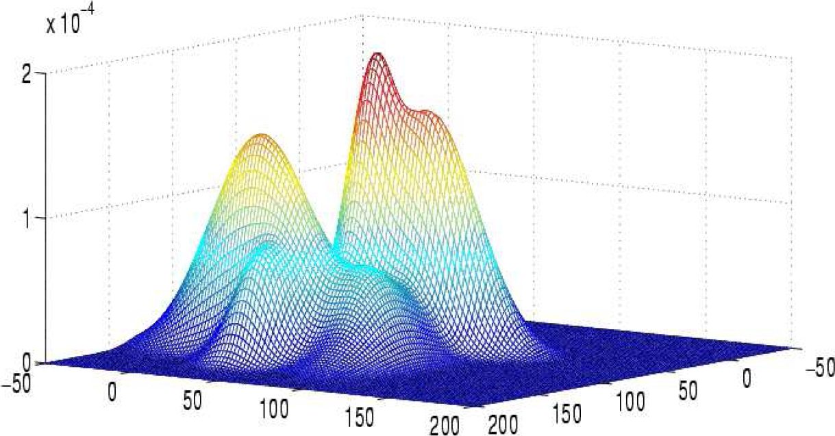
Fig. 2 Overlap Between Three Components of the Mixture in the Three Cases. (a): Total overlap between Γ1 (0.3, 60, 40, 23, 12, 0.3), Γ2 (0.3, 72, 64, 23, 12, 0.2) and Γ3 (0.4, 110, 55, 15, 15, 0.5); (b): Maximum overlap between Γ1 (0.3, 60, 40, 23, 12, 0.3), Γ2 (0.3, 72.69, 64.15, 23, 12, 0.2) and Γ3 (0.4, 110.15, 58.13, 15, 15, 0.5); (c): Partial overlap between Γ1 (0.3, 60, 40, 23, 12, 0.3), Γ2 (0.3, 74.59, 69.27, 23, 12, 0.2) and Γ3 (0.4, 117.58, 63.63, 15, 15, 0.5) 

It is meaningless to evaluate clustering algorithms on total overlapped structures.

Two components in a case of total overlap indicate that these two components form a unique component having different distribution parameters, hence it important to avoid this case.

3.2 Overlap Between Two Equivalent Bivariate Gaussian Components

In order to control components overlap, a formal quantification is needed.

In a bivariate space, let us consider two components Γ1(μx1,μy1,σx,σy,ρ1) and Γ2(μx2,μy2,σx,σy,ρ2), where (μx1,μy1) and (μx2,μy2) represent the centers of the first and the second components. σx and σy represent the standard deviations along each axis; ρ1 and ρ2 are the correlation coefficients and satisfy the equality |ρ1|=|ρ2|.

For two equivalent components, we propose the following condition for the maximum overlap:

Γ1(xint,yint)=Γ20.52πσxσy1ρ2e1/2, (4)

where (xint,yint) represents the coordinate of the highest intersection point that has the highest value. Figure 3 illustrates the three situations related to our condition. In figure 3 (a), the value at the intersection point is higher than the value of the condition given in equation (4), which is indicative of a case of total overlap; it is impossible to visually distinguish between the two mixture components. In figure 3 (b), the intersection point obeys the condition (4). We consider this situation as the case of maximum overlap or a limit case between the total and the partial overlap. In figure 3 (c), it is clear the mixture consists of two components. The two components are in partial overlap.

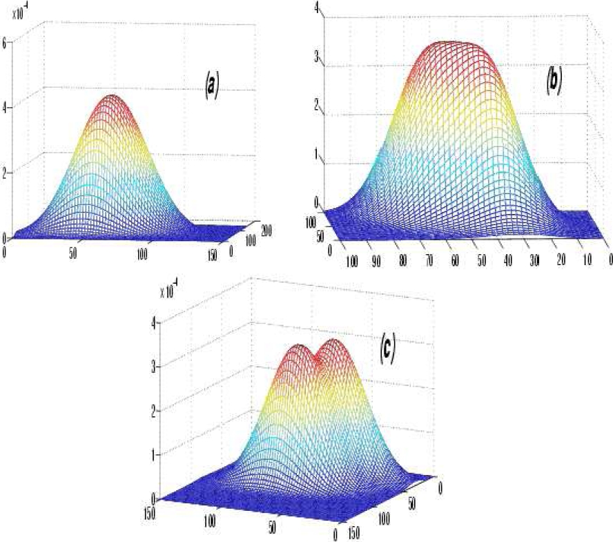
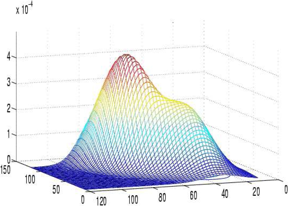
Fig. 3 Generalization and illustration of the condition (3) for two mixture equivalent components. (a) Total overlap: Γ1 (0.5, 60, 40, 23, 12, 0.3) and Γ2 (0.5, 72, 62, 23, 12, 0.3); (b) Maximum overlap: Γ1 (0.5, 60, 40, 23, 12, 0.3) and Γ2 (0.5, 74.86, 64, 23, 12, 0.3); (c) Partial overlap: Γ1 (0.5, 60, 40, 23, 12, 0.3) and Γ2 (0.5, 78, 66, 23, 12, 0.3) 

The value at the intersection point is lower than the value given in condition (4). This results form a relationship between the visual inspection and the formal quantification. We will propose in the next section a definition characterizing the overlap cases. In the rest of this paper, we will use the notation Γi(κi,μxi,μyi,σxi,σyi,ρi) to describe the parameters of the ith component Γi where κi denotes the mixture coefficient, (μxi,μyi) are the coordinates of the components’ centers, σxi and σyi are the standard deviations, ρi is the coefficient of correlation between the two component dimensions and Si=κi2πσxiσyi1ρi2e1/2.

4 Formal Quantification of the Overlap

We propose the definition of the maximum overlap. Later we formalize the degree of overlap by the notion of rate. This definition is similar to that proposed in [17] except that in our case, the definitions are more general in order to support correlated and uncorrelated data. The overlap between components must be controlled to avoid the case of total overlap. We consider the overlap only between the two adjacent components. We will exploit the results of the previous section to propose the definitions.

4.1 Maximum Overlap

The maximum overlap is considered as a limit between the undesirable case of total overlap and the case of partial overlap. The condition of equation (4) is extended to support non-equivalent components and we set the following definition.

Definition 2: Two adjacent Gaussian bivariate components Γ1 and Γ2 are in case of maximum overlap if the value at the highest intersection point Γ1(xint,yint)=min(S1,S2). Figure 4 illustrates an example of maximum overlap between two Gaussian components.

Fig. 4 Example illustrating the maximum overlap between two bivariate Gaussian mixture components, Γ1 (0.4, 60, 40, 23, 12, 0.3) and Γ2 (0.6, 88.27, 69.27, 23, 12, 0.6) 

4.2 Rate of Overlap

In the literature, the notion of overlap is not quantified in a way that an artificial data can be constructed. On the other hand, there are many indices proposed to measure the shared observations or resemblance between clusters. For the most popular model, the Gaussian model, an interesting description of the fretquently used indices for computing the overlap rate between clusters is presented in [12, 32]. The Mahalanobis distance, DMah=((μ1μ2)TΣ1(μ1μ2))1/2, assumes that the two clusters have the same covariance matrix and the same mixture coefficients [16]. The Bhattacharyya distance is an extension of the Mahalanobis distance, DBhatt=18(μ1μ2)T[Σ1+Σ22]1(μ1μ2)+12ln|Σ1+Σ2||Σ1||Σ2| [7]. It is difficult to use such an index because of its computing complexity, so it replaced by its upper bound BBhatt=α1α2eDBhatt in practical applications [16]. Other measures use the PDF to extract a measure for the overlap and similarity between clusters, for example the Kullback-Leibler distance Dkl=p1(x)ln(p1(x)p2(x)dx) [21]. The major inconvenience of this kind of index is that it is not symmetric. The proximity measures presented are relative and assume some conditions on the data which are in most cases simply not verified (like the equality of the components’ coefficients or matrix covariance).

We propose the definition of overlap rate λ by modeling the partial overlap. This concept is based on the following points:

  • — The rate of overlap takes values between 0 and 1, so that the value of 1 implies the presence of maximum overlap and the value of 0 implies that the two components are ”well separated”.

  • — The overlap rate must include all the parameters of the two components: the mixture coefficients, the centers, the standard deviations and the coefficients of correlation.

Definition 3: The rate of overlap between two adjacent bivariate Gaussian components is defined as the ratio of the value at the highest intersection point to the value at the highest intersection point in the case of maximum overlap. Formally, the rate of overlap can be written as:

λ=min(S1,S2)min(S1max,S2max).

These three definitions are very interesting because they employ visual inspection as a basis for the generation and verification of artificial data. Additionally, the rate of overlap definition involves symmetrically all the parameters of the two adjacent Gaussian components. We propose an algorithm for generating artificial data in order to avoid the case of total overlap and control the overlap rate λ. The parameters of the initial component are randomly generated and the parameters of the second component are computed in accordance with one of the three definitions depending on which case is to be reproduced.

5 Controlling Mixture Overlap

As mentioned above, we randomly generate the parameters of the first component - the mixture coefficients, the standard deviations and the coefficients of correlation with the other components. We also introduce the angles of intersection between the components randomly. The angles of intersection are used to measure the deviation of the intersection points from the x axis. After that, we fix the centers of the components, one at a time, according to the rate of overlap.

5.1 Fixing Partial Overlap Rate

For two components Γ1(κ1,μx1,μy1,σx1,σy1,ρ1) and Γ2(κ2,μx2,μy2,σx2,σy2,ρ2), we know all the parameters of Γ1 and κ2,σx2,σy2,ρ2 and we compute the center of the second component (μx2,μy2) according to the rate of overlap λ. We apply the definition of the overlap rate on the two components. There are two cases: S1S2 and S1<;S2.

Case 1: For Γ1, after applying the overlap rate definition, we find:

Γ1(xint,yint)=S2,

which means that:

Γ1(xint,yint)=A1exp(12(1ρ12)[t112σx12+t122σy122ρ1t11t12σx1σy1])=A2exp(1/2),

where: Ai=κi2πσxiσyi1p12 and i{1,2}. t11=(xintμx1) and t12=(yintμy1).

We have:

a1(xintμx1)2+b1(yintμy1)2+c1(xintμx1)(yintμy1)1=0, (5)

where:

e1=12ln(λκ2σx1σy11ρ12κ1σx2σy21ρ22),a1=1(1ρ12)σx12e1,b1=1(1ρ12)σy12e1,c1=2ρ1σx1σy1(1ρ12)e1. (6)

From the inequality S1S2, we conclude that κ1σx1σy11ρ1κ2σx2σy21ρ2. This means that 0<;κ2σx1σy11ρ12κ1σx2σy21ρ221. With 0<;λ1, it is clear that e1>0. So, we deduce that a1 and b1 are also strictly positive.

For the second component, by applying the same reasoning, we find:

a2(xintμx2)2+b2(yintμy2)2+c2(xintμx2)(yintμy2)1=0, (7)

where:

{e2=12ln(λ),a2=1(1ρ22)σx22e2,b2=1(1ρ22)σy22e2,c2=2ρ2σx2σy2(1ρ22)e2. (8)

e2, a2, b2 are also real and strictly positive.

Case 2: In this case, we find the same equations (5,7), but with these parameters for the first component:

e1=12ln(λ),a1=1(1ρ12)σx12e1,b1=1(1ρ12)σy12e1,c1=2ρ1σx1σy1(1ρ12)e1. (9)

and these parameters for the second component:

e2=12ln(λκ1σx2σy21ρ22κ2σx1σy11ρ12),a2=1(1ρ22)σx22e2,b2=1(1ρ22)σy22e2,c2=2ρ2σx2σy2(1ρ22)e2. (10)

In this case, a1, b1, e1, a2, b2 and e2 are all real and strictly positive.

In the plane defined by the equation (T):z=min(S1,S2), the two equations 5 and 7 are characteristic equations of two ellipses with centers respectively at (μx1,μx2) and (μx2,μx1). This means that fixing the center of the second component fixes the center of the second ellipse. First, we compute the value of the intersection point after we compute the center of the second component. We proceed to some transformations in the referential (R), we will translate the referential after we rotate it so that the major axis of the ellipse will be parallel to the X axis of the new referential.

We proceed to translate the referential (R) by the vector m(μx1,μy1). Equation (5) becomes:

a1xint2+b1yint2+c1xintyint1=0. (11)

We obtain an ellipse which center is the center of referential. After translating the referential, we proceed to the rotation in which the major axis of the ellipse will be parallel to the X axis - let us call this new referential R1. Figure 6 illustrates the referential and the angles used for the rotation. We consider the rotation angle ϕ1. Rotation in a bivariate space is given by:

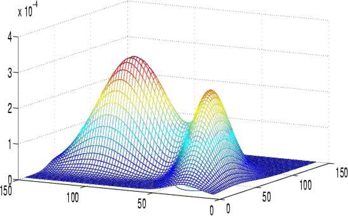
Fig. 5 Partial overlap between two bivariate Gaussian components Γ1 : (0.4, 60, 40, 23, 12, 0.3) and Γ2 : (0.6, 63.67, 98.13, 10, 20, -0.4) with λ = 0.5. 

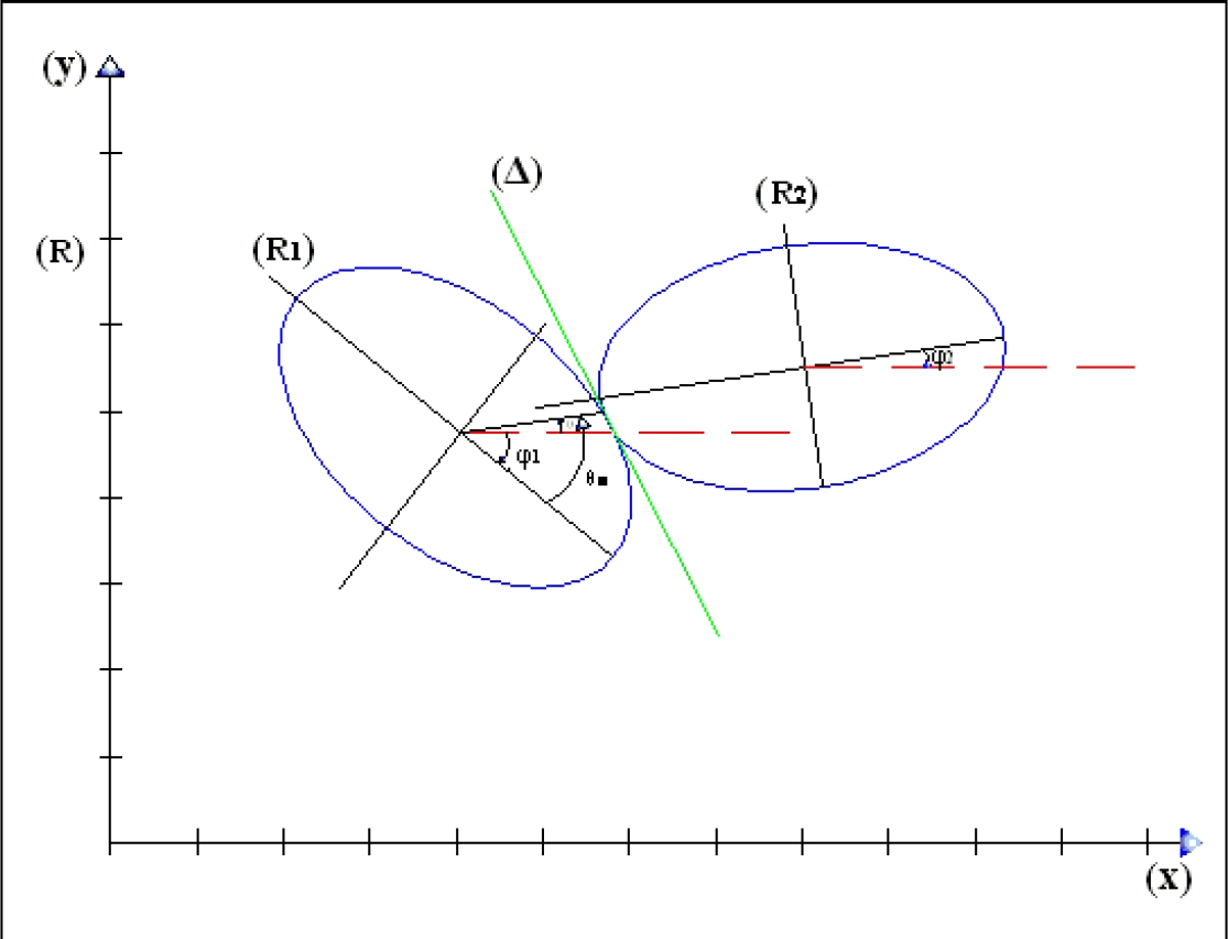
Fig. 6 Illustration of the ellipses’ intersection, the different references and the angles used for the rotation 

{x=xcos(ϕ1)ysin(ϕ1),y=xsin(ϕ1)+ycos(ϕ1), (12)

where x, y are the coordinates in the new referential. To have a referential in which the major axis of the ellipse is parallel to the x axis, the characteristic equation of the ellipse must have the following form in the new referential:

a1x+b1y1=0, (13)

where a1 and b1 are real and strictly positive because the rotation function is isometric: it preserves the distance which means that the ellipse stays an ellipse after rotation.

From equations 11, 12, and 13 and after some transformations, we have:

ϕ1=0.5arctan(c1b1c1),b1=b1cos2(ϕ1)a1sin2(ϕ1)cos(2ϕ1),a1=a1cos2(ϕ1)b1sin2(ϕ1)cos(2ϕ1), (14)

where the angle θ, chosen by the user, represents the deviation of the intersection point Pint from the X axis. The intersection angle θint is used for two reasons. The first one is to fix one solution for computing the center of the second component as there are an infinity of solutions in which the intersection point satisfies the condition imposed by the overlap rate; the second reason is to avoid the ternary overlap between three components. The intersection angle in the new referential (R1), after the rotation, is given by:

{θint=ϕ1+θ,if θintπ/2 then θint=4π/10,if θintπ/2 then θint=4π/10. (15)

To avoid the ternary overlap, Pint is treated in the interval ]π/2,π/2[. For this reason, we add the two conditions cited in the equation (15) and we choose the interval [4π/10,4π/10] as a limit. In [17], there are no conditions on the intersection point interval because, for uncorrelated data, the mixture components have by definition their axes parallel to the referential axis and there is no need for rotation; the intersection angle θint is always within the interval ]π/2,π/2[. From the parametrical equation of the ellipse, Pint coordinates x1 and y1 in the referential (R1) are given by:

{t=arctan(ba1tan(θint)),x1=cos(t)a1,y1=sin(t)b1. (16)

In order to compute the second component’s center, we need the value of the obliqueness at the intersection point. The obliqueness tangent is the tangent of the angle between the line tangent at the intersection point and the X axis. We have three cases; case 1: θint]0,π/2[; case 2: θint]π/2,0[ and case 3: θint=0. For the first case, the function representing this ellipse is given by:

f(x)=1a1x2b1.

The value of the tangent obliqueness δ1 in Pint is:

δ1=a1x1b11a1x12. (17)

For the second case, we find that the function presenting this part of ellipse is:

f(x)=1a1x2b1,

and the obliqueness of the line tangent on Pint is:

δ1=a1x1b11a1x12. (18)

For the third case, where θ=0, the value of the tangent obliqueness δ=. The direction vector of the tangent is parallel to the Y axis. In this situation, there is no need to compute the obliqueness tangent.

Pint(x0,y0) coordinates and the obliqueness of the tangent δ0 in (R) are computed as:

{x0=x1cos(ϕ1)y1sin(ϕ1)+μx1,y0=x1sin(ϕ1)+y1cos(ϕ1)+μy1,δ0=sin(ϕ1)+δ1cos(ϕ1)cos(ϕ1)δ1sin(ϕ1). (19)

In (R1), the direction vector of line tangent is v(1,δ1). We apply the rotation function to v to obtain:

{vx=cos(ϕ1)δ1sin(ϕ1),vy=sin(ϕ1)+d1cos(ϕ1),

where vx and vy are the coordinates of the direction vector after the rotation. The obliqueness is δ0=vyvx.

We proceed to compute the intersection point Pint and the tangent. After some transformation to the tangent line at the intersection point, we extract the coordinate of Pint in a new referential (R2). The new referential (R2) has as origin the center of the second ellipse, and its axes are parallel to the axes of this ellipse. Next, the second mixture component center (μx2,μy2) is derived in the referential (R).

The treatment of the second ellipse is identical to that of the first ellipse (result of the projection of the component onto the xy plane). The referential (R) is translated by the translation vector v(μx2,μy2).

We compute the angle ϕ2 so that the resultant referential (R2) has an axis X parallel to the major axis of the second ellipse. After these transformations, we have:

{ϕ2=0.5arctan(c2b2c2),b2=b2cos2(ϕ2)a2sin2(ϕ2)cos(2ϕ2),a2=a2cos2(ϕ2)b2sin2(ϕ2)cos(2ϕ2), (20)

where the strictly positive real numbers b2 and a2 verify that the resultant characteristic equation of the second ellipse after the rotation is:

b2y2+a2x2=1.

The value of the line obliqueness δ2 in (R2) is given by:

δ2={cos(ϕ2)sin(ϕ2), if (θint=0),sin(ϕ2)+δ0cos(ϕ2)cos(ϕ2)δ0sin(ϕ2), otherwise (21)

For the special case where θint=0, the obliqueness tangent δ0= (the direction vector is parallel to the referential Y axis). It is easy to compute δ2 by rotating the direction vector V(1,0). The intersection point is finally given by: (x2,y2) in (R2):

{x2=δ22bδ22b2a2+a22,y2=1a2x22b2 if δ2<;0,y2=1a2x22b2 if δ2>0. (22)

x2 can take positive values but in order to ensure that there is no total overlap between adjacent components, we choose the negative values.

We compute the coordinates x2 and y2 in (R) on function of μx2 and μy2 by applying the inverse rotation with ϕ2 and by translating with l(μx2,μy2) afterwards. Finally, μx2 and μy2 are given by:

μx2=x2cos(ϕ2)y2sin(ϕ2)+x0,μy2=x2sin(ϕ2)+y2cos(ϕ2)+y0. (23)

It is possible to substitute λ=1 in the previous development to get the maximum overlap, which is a particular case of the partial overlap. Figure 7 shows five mixture components in case of maximum overlap.

Fig. 7 Maximum overlap between five components of the mixture 

By applying the definition of well separated components to the two components Γ1 and Γ2, we have:

a1(xintμx1)2+b1(yintμy1)2+c1(xintμx1)(yintμy1)1=0,

where:

{e1=16,a1=1(1ρ12)σx12e1,b1=1(1ρ12)σy12e1,c1=2ρ1σx1σy1(1ρ12)e1. (24)

For the second component, we find that:

a2(xintμx2)2+b2(yintμy2)2+c2(xintμx2)(yintμy2)1=0, (25)

where:

{e2=10.5ln(λ),a2=1(1ρ22)σx22e2,b2=1(1ρ22)σy22e2,c2=2ρ2σx2σy2(1ρ22)e2. (26)

The two equations 24 and 26 are characteristic equations of two ellipses in the plane (T):z=0. We follow the same equations to find the coordinates of the second component center (μx2,μy2) that satisfies components well separatedness.

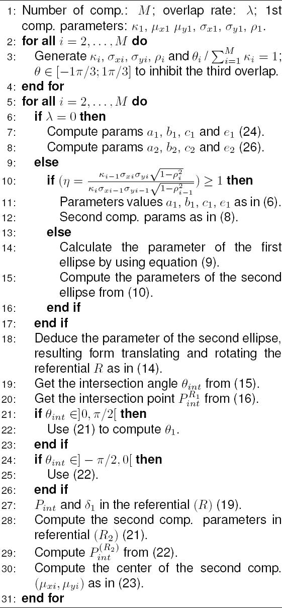
6 Generation Algorithm for Gaussian Bivariate Artificial Correlated Data

In this section, the algorithm of generation of the artificial data is summarized. The general algorithm starts by introducing random values to the parameters of the first component.

We also introduce the mixture coefficients, the standard deviations of the components, the coefficient of correlation and the deviation angles of the other components. The components’ centers are derived afterwards.

In order to avoid the overlap between three components, we suggest to introduce the deviation angles θ in the interval ]1π/3,1π/3[. We suggest also an interval of generation ]1,σmax[ for the standard deviations.

Figures 8 and 9 show a mixture of four components for each rate of overlap. If we exclude the centers of the components, the mixture components have the same parameters. Table 1 shows the generator initializations. The columns represent the mixture coefficients κi, the first dimension standard deviation, the second dimension standard deviation, the correlation coefficient and the intersection angle θint. θint in the table represents the angle between the current component and the next one. These parameters are obtained by varying the rate of overlap to take the values of 0, 0.5, 0.75 and 1.

Fig. 8 Mixture of 4 components. Overlap rate of 1 and 0.75. Density and distributions 

Fig. 9 Mixture of 4 components. Overlap rate of 0 and 0.5. Density and distributions 

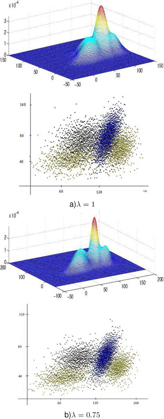
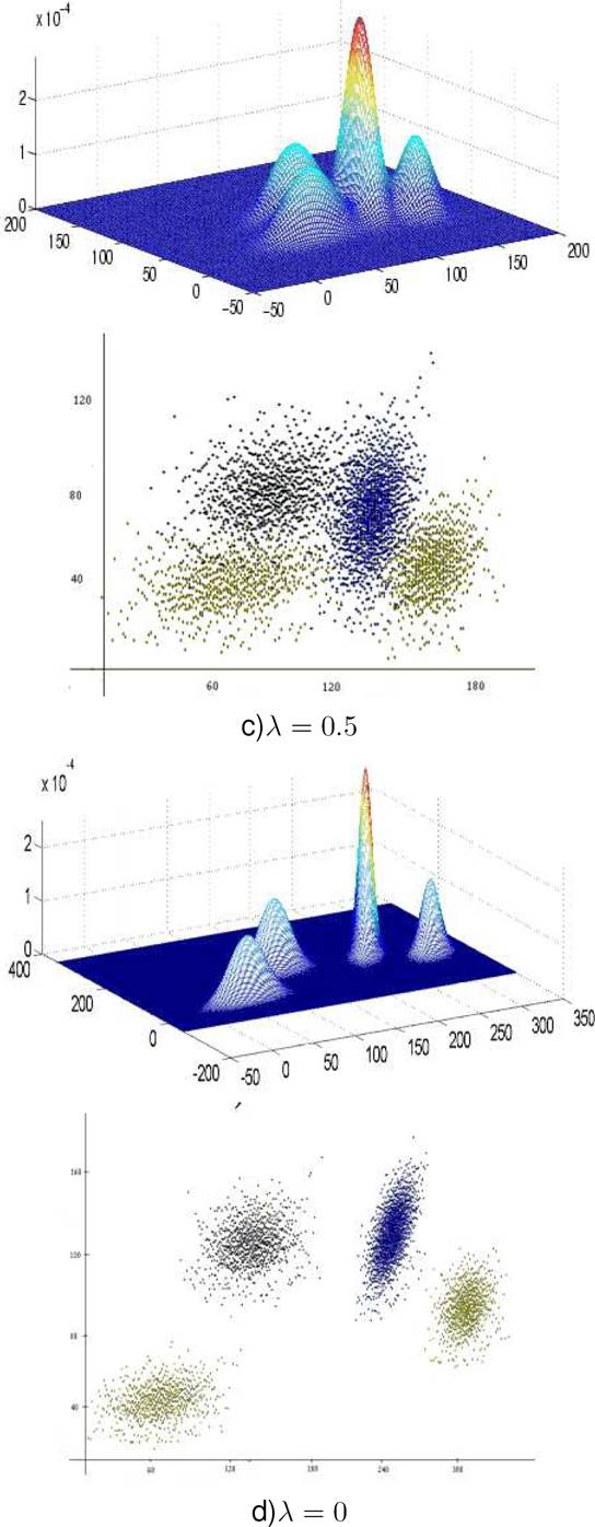
Table 1 Generator initialization to obtain mixture of four components according to the variation of the overlap rate 

mixt coef σxi σyi ρi angle
comp 1 0.25 23 12 0.3 1.016
comp 2 0.25 25 20 0.2 0
comp 3 0.35 15 15 0.4 -1.016
comp 4 0.15 15 20 -0.2

We choose to give the same first component center μ1=(60,40) for each of the experiments.

Table 2 illustrates the centers computed by the generator according to the different overlap rate values. Figures 8 and 9 show both the probability density function pdf and the density scatter plots. We can clearly observe that the scatter approaches each other as λ moves towards 1. It is also shown in [17] an example of four component mixture by varying λ values; however, in the current work, the example is more general, as it is based on a general algorithm and includes unconstrained Gaussian bivariate artificial correlated data.

Table 2 The centers obtained after the generation of bivariate artificial data 

λ 0 0.5 075 1
comp. 1 μx1 60 60 60 60
μy1 40 40 40 40
comp. 2 μx2 111.34 82.50 79.25 76.53
μy2 167.97 93.74 85.23 77.95
comp. 3 μx3 241.93 143.40 133.05 125.63
μy3 159.82 87.97 79.47 71.80
comp. 4 μx4 327.64 186.94 172.74 163.47
μy4 129.27 73.46 66.5 59.89

Algorithm 1 Bivariate correlated Gaussian mixture 

7 Experimental Results

In this section, we present the experimental protocol and results. We propose to use k-Means, Fuzzy C-Means (FCM) and FCM-based splitting Algorithm (FBSA) [27, 19]. For validity indices, we propose to use R-Square (RS), Partition Coefficient (PC), Davies-Bouldin (DB), Xie-Benie (XB), WSJ and Classification Entropy (CE) [40].

7.1 Determination of the Number of Components

As mentioned previously, the influence of the overlap rate on clustering results is discussed. The ability of the clustering methods and the validity indices to determine the number of components is also examined.

In order to give equal opportunity to all the clustering methods to reach the correct cluster structure, we use a unique configuration for choosing the initial centers. We arrange the set of observations according to the first dimension. The kth element is assumed to be the center of the kth cluster so that k=N/C+g where N represents the number of observations, C the number of clusters and g=NmodC. Tables 3 and 4 show the experimental results obtained by the proposed algorithm for 3 components and 5 components, respectively.

Tables 3 and 4 illustrate the results obtained by the proposed algorithm.

The first column represents the clustering methods used in this study: FCM, FBSA and K-Means. The second column contains the value of validity indices RS, PC, DB, XB, WSJ and CE. For each components’ number, we compute the result in group according to the rate of overlap λ{0,0.5,0.75,1}. Figures 8 and 9 represent the constructed data in form of clusters. As seen in Tables 3 and 4, we can easily observe that the indices RS, PC and WSJ give always the same results which means that these indices are not monotonous. For a number of observations which is sufficiently large relative to the number of components, these indices do not produce decent results.

In previous contributions [26, 17], we obtained the same result for the uni-variate and uncorrelated data. In [33], a study concerning the WSJ is presented. It is based on Bersdak suggestion, where the number of observations N=Cmax. The proportion N/Cmax in that study assures good results but in our case where the number of observations N=3000, it’s clear that WSJ is not monotonous. For the same reason, PC and RS aren’t monotonous.

We also show that by increasing the number of components or the overlap rate, the quality of the results decrease. If we look at the experimental results in Table 3, we observe that the validity indices DB, XB, PC determine the component number to be 3, but with the same overlap rate in Table 4 the above validity indices do not have the ability to identify the true number of components.

Table 3 Results for three components 

3 components
λ=0
rs pc db xb wsj ce
fbsa 2 10 3 3 10 3
fcm 2 10 3 3 10 3
db rs
k-means 3 2
λ=0.25
rs pc db xb wsj ce
FBSA 2 10 3 3 8 3
FCM 2 10 3 3 8 3
db rs
k-means 3 2
λ=0.5
rs pc db xb wsj ce
FBSA 2 10 4 10 10 2
FCM 2 10 4 9 10 2
db rs
k-means 2 2
λ=0.75
rs pc db xb wsj ce
FBSA 2 10 2 2 10 2
FCM 2 10 2 2 10 2
db rs
k-means 2 2
λ=1
rs pc db xb wsj ce
fbsa 2 10 2 2 8 2
fcm 2 10 2 2 10 2
db rs
k-means 2 2

Table 4 Results for 5 components 

5 components
λ=0
rs pc db xb wsj ce
fbsa 2 10 5 2 10 3
fcm 2 10 5 2 10 2
db rs
k-means 2 2
λ=0.25
rs pc db xb wsj ce
fbsa 2 10 3 3 8 3
fcm 2 10 3 3 8 3
db rs
k-means 3 2
λ=0.5
rs pc db xb wsj ce
fbsa 2 10 3 3 10 3
fcm 2 10 3 3 10 3
db rs
k-means 2 2
λ=0.75
rs pc db xb wsj ce
fbsa 2 10 2 2 10 2
fcm 2 10 7 8 10 2
db rs
k-means 2 2
λ=1
rs pc db xb wsj ce
fbsa 2 10 2 2 10 2
fcm 2 10 2 2 10 2
db rs
k-means 2 2

A large number of components means that there are relatively a large number of global minima to locate, so that between these global minima a large set of local minima exist where the clustering methods could wrongly converge.

From Table 3, we can easily observe that the determination of the component number becomes less and less accurate as the overlap rate increases.

From the results illustrated in Table 3, we find that all the non-monotonous validity indices are able to find the number of components when the overlap rate λ=0; but, none of them can find the exact number of components with an overlap rate λ=1. These results are confirmed by examining Table 4.

Contrary to the 1D experiences presented in [26], the process of clustering, in this case, cannot converge towards the true models. The curse of dimensionality affects the process for two main reasons. The first one concerns the frequency of dispersion of the data.

For the same number of observations, in 1D space, the data is distributed only on one dimension which causes the data to be more compact and the pdf appears as a continuous function with fewer local minima. However, in 2D, the data is distributed on two axes. Analytically, these spaces are viewed as local minima, and in the pdf representation, they appear as noise. The second reason concerns the overlap between more than two adjacent components.

In [26], in 1D, it is confirmed that the worst situation in which clustering methods encounter difficulty in determining the exact components number is the one where there is a component with a small deviation between two components with large standard deviations. In these circumstances, the first component overlaps beyond the second adjacent component and reaches the third component.

In 2D, there are more chances of such ternary overlap. Suppose we have three 2D components such that the intersection angle between the first and the second components is θint=0.45π, and the intersection angle between the second and the third components θint=0.45π.

In this situation, the first component is so close to the third component that they are in case of total overlap. For this reason, we limited the intersection angles to be within ]π/3,π/3[, despite the fact that this makes it more difficult to control in 2D.

7.2 Determination of the Clusters’ Centers

In this section, we study the ability of clustering methods to determine the model parameters by knowing the number of components. The model parameters includes the mixture coefficients, the centers, the standard deviations and the correlation coefficients. The most important parameter is the centers because a small deviation from its real value has a significant influence on the other parameters.

Another point to take into consideration is that a given deviation of the components centers in the case of minimal overlap does not have the same influence in the case of maximum overlap. Because the data in maximum overlap is more compact, an error which appears negligible in minimal overlap case results in significant divergence in the mixture parameters in the maximum overlap case.

For these reasons, we have introduced a new measure ERavg for computing the deviation of the mixture parameters form the real parameters. ERavg is given by:

ERavg=i=1nc(μxiCxi)2+(μyiCyi)2ncdmax,

where nc represents the number of clusters; μxi and μyi are the coordinates of the ith component; Cxi and Cyi symbolize the ith cluster coordinates; and dmax is the maximum distance between two components centers.

Before computing ERavg, we must first associate each component center to a cluster center. There are two ways to do this. The first is to associate each component center to the nearest cluster center.

The second is to minimize the function defined as minμiμ,CjCd(μi,Ci), where μi is the ith component center, μ is the components centers set, and d(a,b) is the Euclidean distance between a and b. Both methods produce similar results if the errors in centers are relatively small. But, in cases where the deviations in centers are large, the second method is more robust and provides better results. We use the same mixture that we used for the determination of the number of components. Table 5 illustrates the results.

Table 5 Results ERavg of clustering methods 

2 clusters
λ 0 0.25 0.5 0.75 1
k-means 0.03 0.15 0.18 0.13 0.24
fcm 0.0205 0.024 0.0678 0.11 0.16
3 clusters
λ 0 0.25 0.5 0.75 1
k-means 0.007 0.006 0.015 0.0178 0.0185
fcm 0.0025 0.0040 0.0055 0.007 0.0762
4 clusters
λ 0 0.25 0.5 0.75 1
k-means 0.12 0.11 0.0723 0.0705 0.053
fcm 0.0812 0.00421 0.0051 0.00822 0.00842
5 clusters
λ 0 0.25 0.5 0.75 1
k-means 0.00052 0.00481 0.0052 0.041 0.0026
fcm 0.0012 0.00551 0.015 0.0017 0.0183
6 clusters
λ 0 0.25 0.5 0.75 1
k-means 0.054 0.0077 0.0033 0.049 0.018
fcm 0.044 0.0018 0.0241 0.035 0.032
7 clusters
λ 0 0.25 0.5 0.75 1
k-means 0.004 0.0087 0.01 0.013 0.0048
fcm 0.004 0.00465 0.00612 0.0086 0.012

The results are proportional to the overlap rate. As the overlap rate increases, the ERavg increases. In Table 5, for 5 clusters we see that ERavg=0.0012 when λ=0 and ERavg=0.0183 when λ=1.

A large value of λ means that there are many shared observations between data which makes the process of finding the true clusters more difficult. For the same reason, we find that increasing the number of components also increases the ERavg.

8 Conclusion and Future Work

We have proposed an artificial data generator for evaluating the performance of clustering methods. The generator is used to produce artificial data for the mobile centers methods. It also benefits the hierarchical methods where the number of observations is relatively important.

Our approach is based on a formal definition and quantification of mixture components overlap. These definitions are extracted by a formal method in order to have a relationship between visual inspection of the overlap and its formal representation. We have selected three clustering algorithms to be benchmarked (FCM, FBSA and K-Means) and the validity indices RS, PC, DB, XB, WSJ and CE are used in this study.

The experiments are conducted under the same conditions including the initialization parameters and the artificial mixtures. The experimental results have shown the effectiveness and the accuracy of the produced observations especially when the overlap rate increases between components: some algorithms and validity indices outperform others and the monotonic nature of the validity indices is confirmed.

Acknowledgements

This work was funded by a Taif University Research Grant 1-437-5159. The authors are grateful to Taif University Deanship of Research for the institutional support.

References

1.  1. Aitnouri, E., Wang, S., & Ziou, D. (2000). On comparison of clustering techniques for histogram pdf estimation. Pattern Recognition Image Analysis, Vol. 10, No. 2, pp. 206–217. [ Links ]

2.  2. Aitnouri, E., Wang, S., Ziou, D., Vaillancourt, J., & Gagnon, L. (1999). Estimation of a multi-model’s pdf using a mixture model. Neural Parallel Scientific Computation, Vol. 7, No. 1, pp. 103–118. [ Links ]

3.  3. Anderberg, M. (1973). Cluster Analysis for Applications. New York: Academic Press. [ Links ]

4.  4. Baudry, J., Raftery, A., Celeux, G., Lo, K., & Gottardo, R. (2010). Combining mixture component for clustering. Journal of Computational and Graphical Statistics, Vol. 19, No. 2, pp. 332–353. [ Links ]

5.  5. Bayne, C., Beauchamp, J., Begovich, C., & Kane, V. (1980). Monte carlo comparisons of selected clustering procedures. Pattern Recognition, Vol. 12, No. 2, pp. 206–217. [ Links ]

6.  6. Blashfield, R. (1976). Mixture model test of clusters analysis: Accurancy of four agglomerative hierarchical methods. Psychological Bulletin, Vol. 83, No. 3, pp. 377–388. [ Links ]

7.  7. Chen, Y., Qiu, L., Chen, W., Nguyen, L., & Katz, R. H. (2002). Clustering web content for efficient replication. Proceedings of the 10 IEEE International Conference on Network Protocols (ICNP’02), pp. 165–174. [ Links ]

8.  8. Chergas, G., Lorena, L., & Santos, R. D. (2018). A hybrid heuristic for the overlapping cluster editing problem. Applied Soft Computing, Vol. 81, pp. 78–88. [ Links ]

9.  9. Cormack, R. (1971). A review of classification. Journal of the Royal Statistical Society, Vol. 134, No. 3, pp. 321–367. [ Links ]

10.  10. Cunningham, K., & Ogilvie, J. (1972). Evaluation of hierarchical grouping techniques: A preliminary stady. The Computer Journal, Vol. 15, pp. 209–213. [ Links ]

11.  11. Das, A., & Sil, J. (2010). Cluter validation methods for stable cluster formation. Canadian Journal of Artificial Intelligence, Machine Learning and pattern recognition, Vol. 1, No. 3, pp. 26–41. [ Links ]

12.  12. Day, N. (1969). Estimating the components of the mixture of two normal distributions. Biometrika, Vol. 56, No. 3, pp. 463–474. [ Links ]

13.  13. Edelbrock, C. (1979). Comparing the accuracy of hierarchical grouping technique: The problem of classifying every body. Multivariate Behav. Res., Vol. 14, No. 4, pp. 367. [ Links ]

14.  14. Everitt, B. (1974). Cluster Analysis. Heinemann Educational [for] the Social Science Research Council. [ Links ]

15.  15. Everitt, B., & Hand, D. (1981). Finite Mixture Distribution. London: Chapman and Holl. [ Links ]

16.  16. Fugunaga, K. (1990). Introduction to Pattern Recognition. 2nd edn, Academic Press. [ Links ]

17.  17. Gharbaoui, R., Ouali, M., & Aitnouri, E. (2011). A mixture model-based 2d data generator for performance with controlled overlap for performance evaluation. Engineering and Technology, Vol. 78, pp. 73–80. [ Links ]

18.  18. Halkidi, M., Batistakis, Y., & Vazirgiannis, M. (2001). Clustering validation techniques. Intelligent Information System. [ Links ]

19.  19. Jacques, J., & Preda, C. (2014). Model-based clustering for multivariate functional data. Computational Statistics and Data Analysis, Vol. 71, pp. 92–106. [ Links ]

20.  20. Kuiper, F., & Fisher, L. (1975). A monte carlo comparison between six clustring procedures. Biometrics, Vol. 31, No. 1. [ Links ]

21.  21. Kullback, S. (1959). Information Theories and Statictics. Willey, New York. [ Links ]

22.  22. Milligan, G. (1980). An examination of the effect of six types of error perturbation on fifteen clustering algorithms. Psychometrika, Vol. 45, No. 3, pp. 325– 342. [ Links ]

23.  23. Milligan, G. (1985). An algorithm for generating artificial test clusters. Psychometrika, Vol. 50, No. 1, pp. 123–127. [ Links ]

24.  24. Milligan, G., & Cooper, M. (1985). An examination of procedures for determining the number of clusters in a data set. Psychometrika, Vol. 50, No. 2, pp. 159–179. [ Links ]

25.  25. Ouali, M., & Aitnouri, E. (2011). Performance evaluation of clustering technique for image segmentation. Computer Science Journal of Maldova, Vol. 18, No. 03, pp. 271–302. [ Links ]

26.  26. Ouali, M., Gharbaoui, R., & Aitnouri, E. (2011). Benchmarking taxonomy for 1d clustering algorithms. System, Signal processing and thier application (WOSSPA 2011), pp. 151–154. [ Links ]

27.  27. Parastar, H., & Bazrafshan, A. (2016). Fuzzy c-means clustering for chromatographic fingerprints analysis: A gas chromatography mass spectrometry case study. Journal of Chromatography A, Vol. 1438, No. 1, pp. 236–243. [ Links ]

28.  28. Qiu, H., Xu, Y., Gao, L., Li, X., & Chi, L. (2016). Multi-stage design space reduction and metamodeling optimization method based on self-organizing maps and fuzzy clustering. Expert Systems with Applications, Vol. 46, No. 1, pp. 180–195. [ Links ]

29.  29. Riani, M., Cerioli, A., Perrota, D., & Torti, F. (2015). Simulating mixtures of multivariate data with fixed cluster overlap in fsda library. Advences in Data Analysis andassification, Vol. 9, No. 4, pp. 461–481. [ Links ]

30.  30. Salem, A. S., & Nandy, K. A. (2009). Developpement of assessment criteria for clustering algorithms. Pattern Analysis Application, Vol. 12, pp. 79–98. [ Links ]

31.  31. Saltos, R., & Weber, R. (2016). A rough fuzzy approach for support vector clustering. Information Sciences, Vol. 339, No. 2, pp. 353–368. [ Links ]

32.  32. Sun, H., & Wang, S. (2011). Measuring the component overlapping in the gaussian mixture model. Data mining knowledge discovery, Vol. 23, No. 3, pp. 479–502. [ Links ]

33.  33. Sun, H., Wang, S., & Jiang, Q. (2004). FCM-based model selection algorithm for determinig the number of cluster. Pattern Recognition. [ Links ]

34.  34. Wang, W., & Zhang, Y. (2007). On fuzzy cluter validity indices. Fuzzy Sets and Systems, Vol. 158, pp. 2095–2117. [ Links ]

35.  35. Wu, K., & Yang, M. (2005). A cluster validity index for fuzzy clutering. Pattern Recognition Letters, Vol. 26, pp. 1275–1291. [ Links ]

36.  36. Yang, M., Chang, S., & Nataliani, Y. (2019). Unsupervised fuzzy model-based gaussian clustering. Information Sciences, Vol. 481, pp. 1–23. [ Links ]

37.  37. Zhang, B., Liu, W., Zhang, H., Chen, Q., & Zhang, Z. (2016). A note on misspecification in joint modeling of correlated data with informative cluster sizes. Journal of Statistical Planning and Inference, Vol. 170, No. 1, pp. 49–63. [ Links ]

38.  38. Zhao, F., Fan, J., & Liu, H. (2014). Optimal-selection-based suppressed fuzzy c-means clustering algorithm with self-tuning non local information for image segmentation. Expert Systems with Applications, Vol. 41, pp. 4083–4093. [ Links ]

39.  39. Zhao, K., & Lian, H. (2016). The expectation maximization approach for bayesian quantile regression. Computational Statistics and Data Analysis, Vol. 96, No. 1, pp. 1–11. [ Links ]

40.  40. Zhu, E., & Ma, R. (2018). An effective partitional clustering algorithm based on new clustering validity index. Applied Soft Computing, Vol. 71, pp. 608–621. [ Links ]

Received: January 01, 2020; Accepted: February 27, 2020

* Corresponding author: Mohammed Ouali, e-mail: mouali@tu.edu.sa

Creative Commons License This is an open-access article distributed under the terms of the Creative Commons Attribution License