


 nueva página del texto (beta)
 Inglés (pdf)
 Artículo en XML
 Referencias del artículo
 Enviar artículo por email
 Citado por SciELO
  Similares en
SciELO
Similares en
SciELO 
 Permalink
1 Introduction
Image segmentation problem is a fundamental task and process in computer vision and image processing applications. It is an important part of image analysis. It refers to the process of partitioning an image into multiple segments.
In computer vision, graph theory has been successfully applied to solve many tasks, ranging from low-level tasks (image segmentation, etc.), to high-level tasks (image classification, etc.).
Graph theory is the study of graphs. A graph is an abstract representation of a set of objects, where several pairs of the objects are connected by links.
Recently, among the many approaches to image segmentation, graph based methods have become a major trend. Recently, several lines of research revolve around the topic of segmentation and the theory of graphs. Our image segmentation tools are based on graphs, which is a rather recent and rapidly expanding area of image processing. The goal is to segment the main objects out of an image using a segmentation method based on graph cuts. Graph based segmentation techniques gaining popularity in recent days.
Medical images have made a great impact on medicine, diagnosis, and treatment. The most important part of image processing is image segmentation.
In this paper, we are interested in graph-oriented methods which turn the problem of segmenting an image into a problem of partitioning a graph. In these methods, image segmentation is modelled in terms of partitioning a graph into several sub-graphs such that each of them represents a meaningful object of interest in the image. The very first step is mapping the image elements into a graph, where the nodes may be pixels, regions, or even user-drawn markers. The graph structure is formed by a set of nodes (also called vertices) and a set of edges that are connections between pairs of nodes.
Graph based approach is gaining popularity primarily due to its ability in reflecting global image properties. The segmentation problem is solved in a spatially discrete space by the efficient tools from graph theory. Indeed, several algorithms based on graph theory have been proposed. In this paper, we have proposed five methods, which are the spectral method, the FCM method, the kernel method, the FH method and the median method.
After the application of these five algorithms, we also proposed another model based on majority vote, which allows us to merge our five proposed models in order to obtain more precise segmentation results. These methods are applied after the over-segmentation of images into super-pixels followed by the transformation of the map of regions to a graph represented by a set of nodes connected by arcs.
We focus our experimental analysis on the fully-annotated MICCAI brain tumor segmentation (BRATS) data set. Medical Image Analysis is essential in order to detect and diagnose the various types of Cancers.
This paper is organized as follows. In Section 2, we discussed the previous works in graph based image segmentation. In section 3, we introduce the methods as well as the partitioning models of the constrained and unconstrained graph applied to the segmentation of images in bipartite and multiclass. In section 4, include the evaluation of the results obtained by the five proposed algorithms as well as our fusion of classifiers. We will rely on the evaluation of the multi-class bipartite classification using both supervised and unsupervised evaluation criteria. We compared also the experimental results and detailed the performance analysis. We validate our ideas methods on real medical images.
2 Related Work
Graph Theory and its concepts have been dominating in image processing research.
Several applications are made to segment an image using partitioning of the graph. Plenty of methods have been proposed. In this section we briefly consider some of the related work that is most relevant to our approach. [1] is based to determine a set of points, called centers, to minimize the mean squared distance from each data point to its nearest center. [2] is based to extract of the eigenvectors: transform the given data in a manner, such that conventional algorithms like k-means can easily detect the correct patterns. [3] is based to find clusters with nonlinear boundaries in the input data space indeed before clustering; points are mapped to a higher-dimensional feature space using a nonlinear function, and then kernel k-means partitions the points by linear separators in the new space. The algorithm in [4] works in an iterative manner by shifting each graph towards the median graph in a neighborhood. [5] is a simple way of bisecting the graph is to start from a vertex and grow a region around it in a breath-first fashion, until half of the vertices have been included. [6] is based on the optimization of a quadratic classification criterion where each class is represented by its center of gravity. [7] is based to divide the graph into two parts only based on a random choice of the first vertex. [8] is based to reduce the size of the graph (i.e., coarsen the graph) by collapsing vertices and edges, partitions the smaller graph, and then un coarsens it to construct a partition for the original graph. [9] has a collective mechanism to extract local minima such as the ant colony algorithm and the evolutionary algorithm.
3 Proposed Models
Graph-based image segmentation techniques generally represent the problem in terms of a graph G = (V, E) where each node 𝐯𝐢 ∈ V corresponds to a pixel in the image and the edges in E connect certain pairs of neighboring pixels. A weight is associated with each edge based on some property of the pixels that it connects, such as their image intensities. The primary theme of this paper is image segmentation applied on medical images.
In this section, we will present the models of partitioning of the graph that we have chosen to apply them on an image. These approaches depend on two very important steps that must be performed later: Over-segmentation of images and graphs transformation.
3.1 Over-Segmentation
Over-segmentation is used to segment an image into K regions called superpixels indeed it allows to have a set of regions of interest to process, without reducing the amount of raw information in the image (See Figure 1). Superpixels [10] have been exploited to aid segmentation in several different guises. In most cases, they are used to initialize segmentation. A superpixel is commonly defined as a perceptually uniform region in the image. A superpixel representation greatly reduces the number of image primitives compared to the pixel representation.

The desired properties of superpixel segmentation depends on the application of interest. Here we list some general properties [10] required by various vision applications:
— Every superpixel should overlap with only one object.
— The set of superpixel boundaries should be a superset of object boundaries.
— The mapping from pixels to superpixels should not reduce the achievable performance of the intended application.
— The above properties should be obtained with as few superpixels as possible.
Specific algorithms can then be applied to these regions based on their content. There are several types of superpixel segmentation like FH, Superpixel GraphCut, Turbopixels and NCuts super-pixel, but in our work, we base on entropy rate superpixels segmentation and SLIC (the simple lineariterative clustering method).
In this paper, we study the superpixel segmentation [10] as a clustering problem. In order to satisfy the above requirements, we present a new clustering objective function, which consists of two terms: the entropy rate of a random walk on a graph; a balancing term on the cluster distribution. The entropy rate favors compact and homogeneous clusters encouraging division of images on perceptual boundaries and favoring superpixels overlapping with only a single object; whereas the balancing term encourages clusters with similar sizes reducing the number of unbalanced superpixels.
3.1.1 Graph Construction: We Map an Image to a Graph
G = (V, E) with vertices denoting the pixels and the edge weights denoting the pairwise similarities given in the form of a similarity matrix.
Our goal is to select a subset of edges A ∈ E such that the resulting graph, G = (V, A), contains exactly K connected subgraphs. In addition, we also assume that every vertex of the graph has a self loop, although they are not necessary for the graph partition problem.
When an edge is not included in A, we increase the edge weight of the self loop of the associated vertices in such a way that the total incident weight for each vertex remains constant [11] (see Fig. 2).

3.1.2 Entropy Rate
We use the entropy rate of the random walk on the constructed graph as a criterion to obtain compact and homogeneous clusters.
The uncertainty of a random variable is measured by entropy H. Entropy of a discrete random variable X with a probability mass function 𝐩𝐗 is defined by:
3.1.3 Balancing Function
We utilize a balancing function that encourages clusters with similar sizes.. Let A be the selected edge set, NA is the number of connected components in the graph, and ZA be the distribution of the cluster membership. For instance, let the graph partitioning for the edge set A be SA = {S1,S2,...,SNA}. Then the distribution of ZA is equal to:
The connected components show the different groups. The balancing function has a higher value for balanced clustering in (a) than at least one balanced equation (b).
3.1.4 Algorithm
Algorithm 1 is a pseudocode of the greedy algorithm.

At the level of our image, we over-segmented with a number of superpixels fixed a priori and that varies with each test according to the parameters used and in order to show the different regions, we randomly colored them.
3.2 Graph Transformation
The second step is to transform our image into a graph, so that each superpixel obtained from the previous result is treated as a node in a graph and edge weight between two nodes are set proportional to the similarity between the pixels. Each superpixel is represented by its center of gravity as illustrated by the following figure:
Then, we created the similarity matrix S which consists of calculating the Euclidean distance between each pair of superpixels X = {𝑥1,𝑥2,…,𝑥𝑛},Y = {𝑦1,𝑦2,…,𝑦𝑛}, for the three RGB matrices. We calculated for each pair of regions, the sum of the differences between their pixels for each element of these colors which is described by the following formula:
3.3 Graph based Image Segmentation
3.3.1 Image Segmentation using Spectral Model
The first image segmentation algorithm based on spectral clustering [2] which clusters data using eigenvectors of similarity matrix. Spectral clustering transforms the original dataset into a new one in a lower-dimensional eigenspace by utilizing eigenvalues and eigenvectors of a similarity matrix derived from the dataset. Then the traditional clustering algorithms can be performed on this new dataset to obtain the final clustering result. In spectral clustering, a neighborhood graph on the data points is first constructed based on some criteria, such as the fully connected graph or the K-nearest neighbor graph. A weighted similarity matrix is then defined, whose (i, j) element 𝑠𝑖𝑗 reflects the similarity between data point 𝑖𝑥 and 𝑗𝑥.
The measuring of the similarity between samples is still an open problem in spectral clustering, and Gaussian kernel function is adopted in most references to measure the similarity of samples.
Many algorithms have been developed that find a reasonably good partition with spectral partitioning, where a partition is derived from the spectrum of the adjacency matrix; there are three types of Spectral clustering algorithm.
Unnormalized Algorithm, Normalized spectral clustering according to Shi and Malik (2000) and Unnormalized spectral clustering according to Jordan and Weiss (2002).
We will present our first contribution, which consists in applying the spectral model to an image, more precisely, we will reapply the standardized cut method of J. Shi and J. Malik, the method weiss_Jordan and the Unnormalized method by modifying the form of the graph used by our new form quoted above. In other words, each vertex will be a superpixel instead of a pixel, and instead the similarity matrix is based on distance and intensity we will only be interested in RGB colors. To activate the procedure, we need as centroid parameters, the similarity matrix and the number of desired parts K.
The idea used in this paper is to perform an over-segmentation of the image, the second step is to transform our image into a graph, so that each superpixel obtained from the previous result is treated as a node in a graph and edge weight between two nodes are set proportional to the similarity between the pixel then use the spectral clustering.
The unnormalized algorithm we just presented used the unnormalized graph Laplacian L, which is why we refer to this algorithm as the unnormalized spectral clustering.Shi and Malik approximate computing the minimum normalized cut criterion with eigen-problem, later, Weiss has shown how the eigenvector problem relate to more standard spectral partitioning methods on graphs.The core idea is to use matrix theory and linear algebra to study properties of the incidence matrix, W, and the Laplacian matrix, L = D − W, which provide a great deal of information about graph G. Using the spectrum of graph Laplacian, which is symmetric positive semidefinite matrix, can capture essential cluster structure of a graph, i.e. the eigenvectors of the graph Laplacian or its variants.
Algorithm 2 is a pseudocode of the Unnormalized algorithm.

Diagram that summarizes the work with the three variants of the spectral algorithm (see Fig. 7).


Fig. 5 We show the role of the balancing function in obtaining clusters of similar sizes. The connected components show the different clusters. (a) The balancing function has a higher objective value for the balanced clustering, (b) compared to the less balanced

Fig. 6 (a)initial image, (b) Lena image over-segmented at gray level with n = 100, (c) Lena image over-segmented in color, (d) histogram

3.3.2 Image Segmentation using (FCM) clustering
Is another popular clustering algorithm that most used in image segmentation problems. An FCM [6] technique introduces the fuzzy concept into image segmentation problems so that an object can belong to several classes as same time. It is an unsupervised technique and it basic idea is that clustering the data points by iteratively minimizing the cost function, which is dependent on the distance between the pixels and the cluster center in the feature space.
We will present our second contribution, which consists in applying the FCM method to an image, modifying the shape of the graph used by our new form mentioned above. In other words, each vertex will be a super-pixel instead of a pixel, and the Euclidean distance of degree of similarity between two region pairs will be calculated through the Euclidean distance between each pair of super-pixels for the three RGB matrices.
Algorithm 3 is a pseudo code of the FCM algorithm.

Diagram that summarizes the work with the three variants of the spectral algorithm (see Fig. 8).

3.3.3 Image Segmentation using Median Graph
The algorithm can serve two goals, either clustering or selecting representative prototypes. In this paper, we draw an evaluation of its clustering application. From a given set of graphs G, the algorithm returns a set of clusters {𝐶𝑗} and each cluster has a representative prototype 𝑝𝑖. The radius h, called bandwidth in the classical meanshift, is a parameter fixed a priori. The algorithm computes the number of cluster during execution.
In the algorithm, first each graph 𝑔𝑖 ∈ G is associated to an empty graph 𝑔𝑚𝑠𝑖. Then, for each graph 𝑔𝑖 ∈ G the inner loop is performed. This loop computes for the graph 𝑔𝑖 a steady median graph 𝑔𝑚𝑠𝑖. We define the steady median graph 𝑔𝑚𝑠𝑖 as the final median graph returned by a shifting series of 𝑔𝑖.
The median graph shift clustering [4] is a deterministic and nonparametric algorithm. It computes the number of clusters during execution. In this part we will present our third contribution, which consists of applying the median graph method to an image, modifying the shape of the graph used by our new form mentioned above.
In other words, each vertex will be a super-pixel instead of a pixel, and the similarity between two region pairs will be calculated through the Euclidean distance between each pair of super-pixels for the three matrices R G B.
Algorithm 4 is a pseudo code of the median graph algorithm.
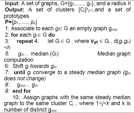
Diagram that summarizes the work with median Graph algorithm (see Fig. 9).

3.3.4 Image Segmentation using FH
This is a very effective graph based method. This method discourses the problem of segmenting an image into regions or segments. A predicate is defined for measuring the indication for a boundary between two regions of an image, using a graph-based representation.
Afterwards, an efficient segmentation algorithm is developed based on this predicate. Felzenszwalb and Huttenlocher’s graph-based method (FH) [12] merges regions greedily, and tends to return gross segmentation.
In this section, we define a predicate, D, for evaluating whether or not there is evidence for a boundary between two components in segmentation (two regions of an image). This predicate is based on measuring the dissimilarity between elements along the boundary of the two components relative to a measure of the dissimilarity among neighboring elements within each of the two components. The resulting predicate compares the inter-component differences to the within component differences and is thereby adaptive with respect to the local characteristics of the data.
We define the internal difference of a component C ∈ V to be the largest weight in the minimum spanning tree of the component, MST(C, E). That is:
We define the difference between two components C1, C2 ∈ V to be the minimum weight edge connecting the two components. That is:
The region comparison predicate evaluates if there is evidence for a boundary between a pair or components by checking if the difference between the components, Dif(𝑪𝟏, 𝑪𝟐), is large relative to the internal difference within at least one of the components, Int(𝑪𝟏) and Int(𝑪𝟐). A threshold function is used to control the degree to which the difference between components must be larger than minimum internal difference. We define the pairwise comparison predicate as:
The input is a graph G = (V, E), with n vertices and m edges. The output is a segmentation of V into components S = (𝑪𝟏),..., 𝑪𝒓).
In this part, we will present our fourth contribution, which consists in applying the FH method to an image, modifying the shape of the graph used by our new form mentioned above.
In other words, each vertex will be a super-pixel instead of a pixel, and the similarity between two region pairs will be calculated through the Euclidean distance for the three matrices R, G, and B.
Pseudo code of the FH algorithm is presented in Algorithm 5.

Diagram that summarizes the work with median Graph algorithm (see Fig. 10).

3.3.5 Image Segmentation using Kernel K-means
Kernel k-means is an extension of the standard k-means clustering algorithm that identifies nonlinearly separable clusters. In order to overcome the cluster initialization problem associated with this method, in this work we propose the global kernel k-means algorithm, a deterministic and incremental approach to kernel-based clustering.
Our method adds one cluster at each stage through a global search procedure consisting of several executions of kernel k-means from suitable initializations.
This algorithm does not depend on cluster initialization, identifies nonlinearly separable clusters and, due to its incremental nature and search procedure, locates near optimal solutions avoiding poor local minima.
Furthermore, a modification is proposed to reduce the computational cost that does not significantly affect the solution quality. This algorithm can be used to optimize monotonically a number of graph clustering objectives.
The weighted kernel k-means algorithm can be used to optimize a wide class of graph clustering objectives such as minimizing the normalized cut.
As a result, the weighted kernel k-means algorithm can be used to optimize a number of graph clustering objectives. This allows us the flexibility of having as input to the algorithm either a graph or data vectors that have been mapped to a kernel space.Kernel k-means is a generalization of the standard k-means algorithm where data points are mapped from input space to a higher dimensional feature space through a nonlinear transformation Φ and then k-means is applied in the feature space.
These results represent linear separators in feature space, which correspond to nonlinear separators in input space. Thus kernel k-means avoids the problem of linearly separable clusters in input space that k-means suffers from.
The objective function that kernel k-means tries to minimize is the equivalent of the clustering error in the feature space shown in. We can define a kernel matrix k ∈ Rn × n where K (𝑥𝑖,𝑥𝑗) = {Φ (𝑥𝑖), Φ (𝑥𝑗)}.
The map of this figure is created using the function we call a polynomial kernel k (𝑥𝑖,𝑥𝑗) = (𝑥𝑖 · 𝑥𝑗 + 𝑐)𝑑.
The explicit map for the polynomial kernel is:
We represent an element of the k-matrix kernel as follows:
Some well-known kernel functions are the polynomial core and the core of the
radial base function
In this part, we will present our fifth contribution, which consists in applying the Kernel method to an image, modifying the shape of the graph used by our new form mentioned above. In other words, each vertex will be a superpixel instead of a pixel, and the similarity between the observations is based on the RGB colors.
Diagram that summarizes the work with FH algorithm (see Fig. 11).


Fig. 15 Test on the effect of the number of regions by the spectral method, (a) Original image, (b) over-segmented Image N = 70, (c) Segmented image N = 70, ( d) over-Segmented image N = 200,(e) Segmented image N = 200

Fig. 16 Test on the effect of the number of regions by the FCM algorithm, (a) Original image, (b, d) over-Segmented image N = 70, 100 respectively, (c, e) Segmented image N = 70, 100 respectively
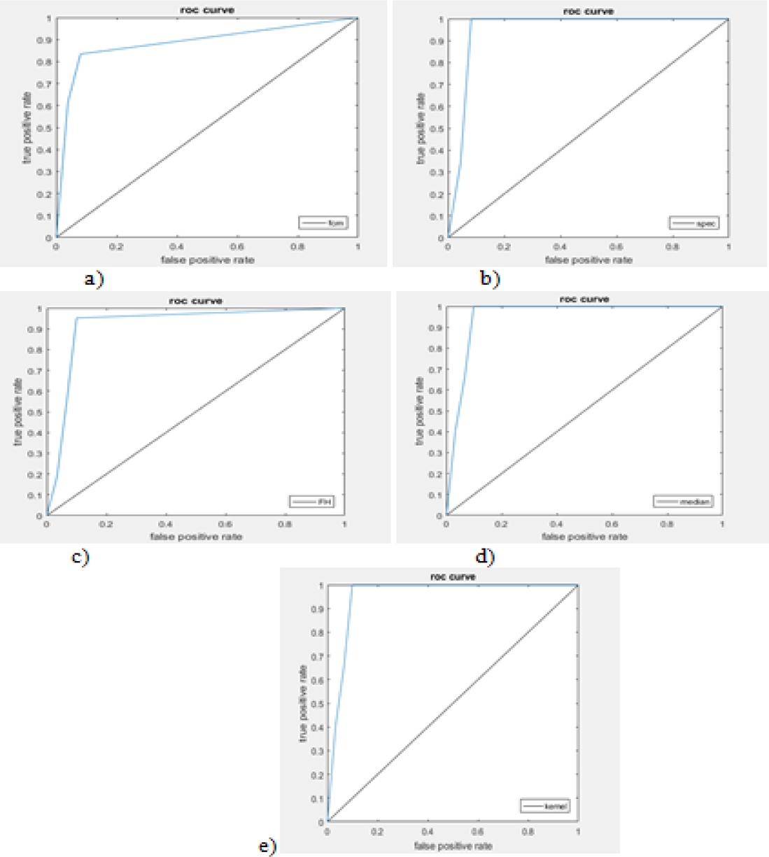
Fig. 17 The ROC curves of the five methods, (a) FCM algorithm; b) spectral algorithm; (c) FH algorithm; (d) Median algorithm, (e) Kernel algorithm respectively with the bipartite segmentation of images

3.3.6 Combination of Classifiers
In this paper, we combine different segmentation methods for image segmentation, which, to our knowledge, has not been sufficiently explored.
We propose a new approach, which enables to fusion either the results of several segmentation methods of a same image or the different results in the case of a multi-components image.
This approach is applied to segment multi-components images by combining the segmentation results of each component. Algorithm 6 is a pseudocode of the Kernel-K-means algorithm.

The proposed fusion principle is an adaptation of the cooperative segmentation method [13].
It has been defined as a segmentation where two or more (two in the proposed segmentation, but the principle is more general) features are simultaneously extracted, requiring explicit transfers of information during the segmentation process. It performs a data fusion between information coming from different feature detectors, namely here edge and region. We have proposed a new weighted combination method for multiple classifiers based on evidential reasoning.
These evidential methods can well handle the uncertainty in pattern classification for achieving a good performance. Proposed approach: Combination of classifiers with majority vote. The method is based on the principle of the parallel combination of distributed systems using majority voting.
Our main contribution is summarized as follows. We combine different segmentation methods: the spectral, FCM, kernel, FH and median. Experimental results show the benefit of this method.
4 Experimental Results
This section shows the experimental evaluation of our proposed algorithms and its results on some images of BRATS [14] data set and standard test image Lenna.

Fig. 19 Segmentation of images with variations of the number of classes: (a) original images, (b) segmented images, (c, d, e) segmented images with k of value: 2,3,5 respectively
4.1 Databases
We used BRATS brain tumor segmentation data set, that contains a lot of images. The experiments were carried out on real patient data obtained from the 2013 brain tumor segmentation challenge (BRATS2013). The BRATS2013 data set is comprised of 3 sub-data sets.
The training data set, which contains 30 patient subjects all with pixel-accurate ground truth (20 high grade and 10 low grade tumors); the test data set which contains 10 (all high grade tumors) and the leaderboard data set which contains 25 patient subjects (21 high grade and 4 low grade tumors).
4.2 Type of Evaluation
Segmentation is a fundamental step in image analysis and remains a complex problem. Many segmentation methods have been proposed in the literature but it is difficult to compare their efficiency. In order to contribute to the solution of this problem, some evaluation criteria [15] have been proposed for the last decade to quantify the quality of a segmentation result.
Supervised evaluation criteria use some a priori knowledge such as a ground truth while unsupervised ones compute some statistics in the segmentation result according to the original image.
4.2.1 Supervised Evaluation
The principle of this approach is to measure dissimilarity between a segmentation result and a ground truth (ideal result).
4.2.2 Unsupervised Evaluation
Without any a priori knowledge, it is possible to quantify the quality of a segmentation results by using unsupervised criteria. Most of these criteria compute statistics on each region in the segmentation result. The majority of these quality measurements are established in agreement with the human perception. For region, segmentation, the various criteria take into account the intra-region uniformity and inter-regions contrast.
One of the most intuitive criteria being able to quantify the quality of a segmentation result is the intra-region uniformity. Weszka and Rosenfeld proposed such a criterion that measures the effect of noise on the evaluation of some thresholded images. Based on the same idea of intra-region uniformity, Nazif and Levine also defined a criterion that calculates the uniformity of a characteristic on a region based on the variance of this characteristic.

Fig. 20 Segmentation of images by the FCM algorithm with variations of the number of classes and the number of homogeneous regions (a, f, k) original images, (b, g, l) segmented images, (c, h, m); (d, i, n); (e, j, f) segmented images with k of value: 2,3,5


Fig. 22 Example of image segmentation lenna, (a) original image, (b) over-segmented image, (c, d) image segmented with two different classes: k = 3, k = 6


Inter-Regions Contrast: Complementary to the intra-region uniformity, Levine and Nazif defined a gray-level contrast measurement between two regions to evaluate the dissimilarity of regions in a segmentation result. The formula of total contrast is defined as follows. Intra- and Inter-Regions Contrast:
Liu and Yang proposed a criterion considering that:
4.3 Evaluation of Bipartite Segmentation
4.3.1 Effect of Over-Segmentation
We have noticed that the number of regions fixed in the over-segmentation step has an influence on the result. So, if the number of classes is concise, preferably the number of regions is concise as well.
Our experiments have been done with different parameter: number of classes fixed and small and different number of regions.
For the second test, if the initial over-segmentation is too coarse, there will be segments that overlap the boundary of the object and lead to incorrect segmentation. In addition, if the over-segmentation is too thin, the number of neighbors of a super pixel will increase significantly. This could influence the spatial interaction between adjacent superpixels and slightly the segmentation performance.
4.3.2 Supervised Evaluation
Evaluation Based on ROC Curves Analysis: This method is based on receiver operating characteristic (ROC) curves. A ground truth is defined by the experts for each image and is composed of three areas.
We will represent the results of the sensitivity calculation, the specificity and the efficiency of each method in the ROC curves. We noticed that different ROC curves converge to 1. We can notice, at the beginning, that the three spectral methods, FCM and kernel have values between 0.8 0.9 and lower than 1. If the value is worth to 1 this method is perfect. Then we found that these three methods are the most efficient compared to the other two methods FH and median which have values lower than 0.8. To reinforce this contribution, we notice that all the values in the three ROC curves are greater than the fixed threshold (0.5) and converge to 1. The following curve summarizes the result of all the algorithms.
4.3.3 Unsupervised Evaluation
Quantitative Analysis
The measurements of this criterion can be evaluated using a threshold equal to 0.5. According to the results obtained in several articles [15] if the value is lower than the threshold then it is a bad segmentation.
According to this definition, we find that the measures of the FCM method are the most remarkable because of their increase compared to the other measures related to the other algorithms. It shows the capacity of this method to be a benchmark. We find that all the values are greater than or equal to 0.5 in kernel method.
Indeed, they are very close to the measures of the FCM method. The same interpretation for the spectral method.
Finally, for the other two methods median and FH we note that their measurements are lower than the measurements of the three previous algorithms.
4.4 Evaluation of Bipartite Segmentation
4.4.1 Effect of Over-Segmentation
Image segmentation into two classes separates the object from the bottom as we obtained in the previous part. But in the case of choosing a large number of classes (K> 2), we can guarantee a surplus of regions in the final segmentation. In other words, the increase in the number of classes brings about the appearance of the details of the image, and the detection of the different intensities of the regions. This number depends on the number of homogeneous regions in the original image as well as the number of superpixels at certain times although it has no influence on the bipartite segmentation. We apply segmentations on the same image with a fixed region number but with a different class number as following.
Spectral Algorithm
We note here that if the number of classes is high, the result of segmentation becomes more precise and we see the appearance of several details concerning our image.
For medical images, if the number of classes is high we observe the appearance of several details of the image.
Kernel Algorithm
First, the variation in the number of regions in the over-segmentation step shows that the higher the number of superpixels the more details of the image have appeared. In such a way the contrast at the contour of the image appears only for N> 70, also for the difference of intensity which is localized in the image is not illustrated only for N> 110.
Thus, the more the number of superpixels increases the more the number of regions must be high, which is shown by the following example, which presents an over-segmented image with n = 100 and two images classified with two numbers of different classes K = 3 and K = 6.
4.4.2 Unsupervised Evaluation of Multi-Classes Segmentation
Quantitative analysis: We will only apply the unsupervised evaluation. Then, we chose the number of classes between 4 and 8 that varies according to the properties of the image to be tested, and the number of super-pixels is between 200 and 500. Each time, we have to calculate the values of the inter, intra and inter-intra regions of each segmentation for each method, which are illustrated in the following:
We find that the measurements are all greater than 0.5 and less than 0.6, which validates the performance of all the methods.
The result of combination of classifiers:
Our test was performed on a Medical image. It has been classified by five different classifiers: the spectral classifier, FCM classifier, FH classifier, Kernel classifier, FCM and the Median classifier. We see an improvement in the combination image compared to the images of the classifiers. The combination result is less noisy than the best result of the five classifiers. The ROC curve shows that the combination of the five classifiers has improved the final result of the combination. Thus, the method proposed here has made it possible to obtain a more precise segmentation.
Image segmentation plays a crucial role in many medical-imaging applications, by automating or facilitating the delineation of anatomical structures and other regions of interest. The table 3 presents the different methods used as well as their performance and complexities. Taking into account the various qualitative parameters, namely the precision and the complexity, the table clearly shows that the proposed method (metaclassifier or fusion method) is the best in terms of compromise. This confirms the current trend in scientific research; the importance and contribution of the fusion of classification techniques.
Table 1 The intra-inter values of the images for each algorithm
Algorithm
|
Unnormalised
K=2 N=200 |
(Shi&Malik) K=2 N=200 |
(Jordan&Weiss) K=2 N=200 |
| Intra | 0.0657 | 0.0490 | 0.0352 |
| Inter | 0.1264 | 0.1013 | 0.1582 |
| Intra_inter | 0.5304 | 0.5261 | 0.5615 |
Algorithm
|
FCM K=2 N=200 |
FH K=2 N=200 |
Kernel K=2 N=200 |
Median K=2 N=200 |
| Intra_inter | 0.5716 | 0.5004 | 0.5708 | 0.5395 |
Algorithm
|
FCM K=2 N=200 |
FH K=2 N=200 |
Kernel K=2 N=200 |
Median K=2 N=200 |
| Intra_inter | 0.5878 | 0.5005 | 0.5664 | 0.5402 |
Algorithm
|
FCM K=2 N=200 |
FH K=2 N=200 |
Kernel K=2 N=200 |
Median K=2 N=200 |
| Intra_inter | 0.5604 | 0.5006 | 0.5639 | 0.5381 |
Table 2 Measurements of the criteria intra- inter- region
Algorithm
FCM
|
K=4; N=200 | K=8; N=200 | K=4; N=500 |
| Intra | 0.0406 | 0.0329 | 0.0355 |
| Inter | 0.1448 | 0.1299 | 0.1575 |
| Intra_inter | 0.5521 | 0.5485 | 0.5610 |
Algorithm
FCM
|
K=4; N=200 | K=8; N=200 | K=4; N=500 |
| Intra | 0.0207 | 0.0172 | 0.0351 |
| Inter | 0.2064 | 0.1416 | 0.1560 |
| Intra_inter | 0.5928 | 0.5622 | 0.5605 |
Algorithm
FCM
|
K=4; N=200 | K=8; N=200 | K=4; N=500 |
| Intra | 0.0120 | 0.0072 | 0.0105 |
| Inter | 0.1380 | 0.1052 | 0.1277 |
| Intra_inter | 0.5630 | 0.5490 | 0.5586 |
5 Conclusion
In this paper, we have proposed five methods based graph theory, which are the spectral method, the FCM, the kernel method, the FH method and the median method. These methods are applied after the over-segmentation of images into super-pixels followed by the transformation of the map of regions in a graph.
After the application of these five algorithms, we also proposed another model based on majority vote. We found that the five approaches are efficient and effective based on the measurements and the results obtained for the segmentation of bipartite and multi-classes images.
We show that these methods are works very well for most of the images. This paper presents to better approach for applications when it is necessary to extract particular objects in e.g. medical images.

