


 nueva página del texto (beta)
 Inglés (pdf)
 Artículo en XML
 Referencias del artículo
 Enviar artículo por email
 Citado por SciELO
  Similares en
SciELO
Similares en
SciELO 
 Permalink
1 Introduction
Reconstructing depth from a single monocular image (opposed to stereoscopic images) is a challenging task due to the required ability to detect depth cues such as shadows, perspective, motion blur, etc. [14]. Previous works in depth reconstruction have tackled the general problem of estimating the component of depth in a wide range of images, mainly focusing on objects against a solid or a complex background [20, 2, 4, 23, 19]; other works focus on city buildings and people, paying special attention to the problem of reconstructing depth for images where perspective plays a predominant role [25].
In general, most successful models in the state of the art—v. gr. [6, 2]—propose multi-stage networks that require separate training for each one of their stages, making the process of training them complex and time consuming. In this paper, we propose five Convolutional Neural Network models capable of reconstructing depth from a single image that require only one training stage. The models proposed in this work are capable of reconstructing depth both in a global and a local view [14]. We test our models with both objects and city roads with perspective.
This paper is organized as follows: in Section 2 we describe related work to this research; Section 3 describes the proposed method; Section 4 shows the results obtained from our proposal and a comparison with the state of the art, and finally in Section 5 the conclusions of this work are drawn.
2 Related Work
Depth reconstruction from a single image has been tackled by different methods. Although using Convolutional Neural Networks (CNN) has recently become one of the best techniques, using CNN to solve the problem of depth reconstruction can be still considered at as a development stage due to the complexity of the design of these networks. One of the first works to use this technique can be found in [7].
They propose using two CNN: the first one estimates depth at global view, and the second one refines the local view. They establish a CNN architecture to be applied to depth estimation and propose a loss function.
In [6] using three CNN is proposed, one for each stage to estimate depth of a single image. The first network estimates depth at a global view; the second network tries to estimate depth at half the resolution of the input image, and a third one refines or estimates depth at a local level. They propose a new loss function. In [20] a single CNN is presented that uses a pre-processed input based on superpixels. They complement their work using a probabilistic method to improve their results. Then, from the same group [21] presents a new architecture of their network maintaining the stage of improvement of the image. Finally, a single CNN in regression mode is presented in [2] to estimate depth with a different loss function.
In general, the discussed architectures are similar, being the main changes between them the loss function, activation functions, number of filters per layer, and size of the filter. Different databases have been used to train and test their neural networks, making it difficult to directly compare their performances. Despite of this, one of the works that can be considered to achieve the best results in the state of the art is [2]. Additionally, their architecture is based on a single-stage CNN. They present results of reconstructing depth of chair images against different backgrounds.
In the next section we present our proposal. Based on Afifi and Hellwich’s CNN, our architec-tures are based on a single CNN, but, among other differences, we add local refinement in the same training stage in most of our models.
3 Proposed Method
In this section we present our models based on Convolutional Neural Neworks (CNN). We have decided to name them according to the kind of layers they use, namely: Convolutional layers (C) [16]; reSidual blocks (S) [11]; Upsample layers (U) [27]; and Refinement layers (R). We also add biases to each layer. In Fig. 1 a representation of a layer in the CNN models is shown.

As mentioned before we implemented Afifi and Hellwich’s CNN model to compare our results, as they perform depth estimation in a single stage, depicted in Fig. 2. They use Convolutional Blocks made by consecutive convolutional layers as shown in Fig. 3.


3.1 Basic Models – Convolutional (C) and reSidual-Convolutional (SC)
In this section we present two CNN models, the first one (C:Convolutional) is presented in Fig. 5 and the second one (SC: reSidual-Convolutional) is presented in Fig. 6. The main differences between both models are the kind of layers used in every layer, one of them only uses convolutional layers and the other one uses residual blocks and convolutional layers.


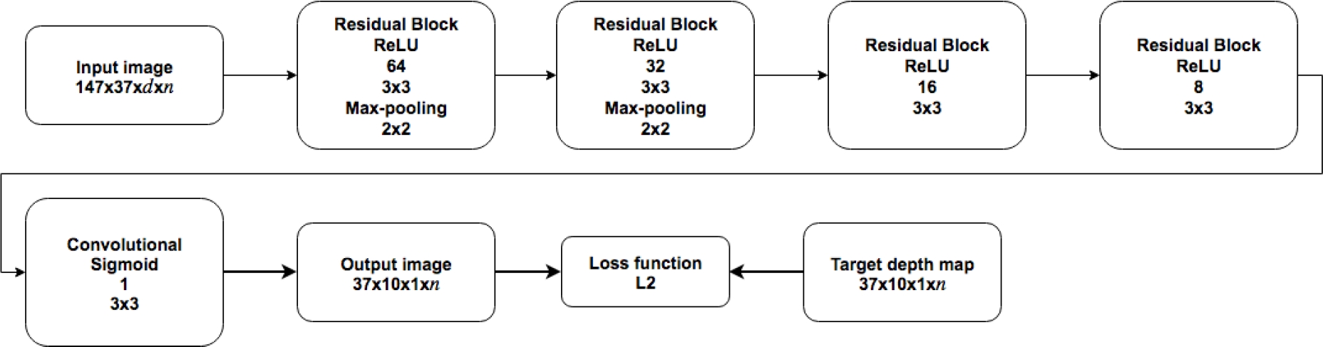
The Residual Block is shown in Fig. 4, it uses an identity map which helps to improve the results as mentioned in [11]. Both models consist of five layers, four of them use Rectified Linear Units (ReLU) [3] as activation function and the output layer uses sigmoid as activation function to obtain values between 0 and 1. In both models the first two layers use max-pooling in order to reconstruct depth at different spatial resolutions of the input image. In every layer of the models the kernel size is 3x3 and subsequently it changes in each layer. Both models reconstruct depth at both global and local.
3.2 Models with Refinement
Aiming to include refinement in a single training stage, we developed three additional models.
The main difference between them is the upsample operation and the refinement method. The refining methods used in the CNN models are based on Xu et al. [26] and Dosovitskiy et al. [5], both refinement methods use convolutional layers to extract features directly from the input images at local level, the main difference between them is the number of convolutional layers and how it is included on the full CNN model, also Xu et al. performs refinement before the upsampling stage and Dosovitskiy performs refinement after the upsampling stage.
3.2.1 reSidual-Convolutional-Refinement (SCRX) Model
The block diagram of this model is presented in Fig. 7. The input image is the left image of the dataset and the
target image is the depth map obtained from the stereo matching algorithm.
In Region A we can see the Reduction operation which tries to reconstruct
depth at global view; it consists of four Residual Blocks with kernel size
of
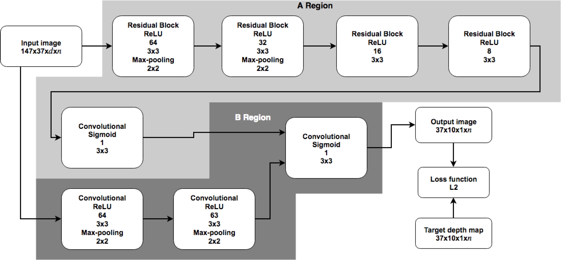
We use Max-pooling only on the first two Residual Blocks to reduce image
resolution and reconstruct depth at different image sizes. At the end of
Region A we use a convolutional layer with a sigmoid activation function to
limit output limits beetween 0 and 1. Region B tries to estimate depth at
local view, joining the output of Region A and two convolutional layers with
Max-pooling. The refining method in this model was taken from the work of Xu
et al. [26]—hence the X in
SCRX. The output of the model is given by the convolutional layer with
kernel size
3.2.2 reSidual-Convolutional-Refinement-Upsampling Models (SCRXU and SCRDU)
These models consist of an additional upsample layer. Two different refining methods were used in each model: the refining method in the first model (SCRXU) is based on [26] and for the second one (SCRDU) is based on [5].
The block diagrams of these models are presented in Fig. 8 and Fig. 9.
The input image is the left image of the dataset [8] and the target image is the depth map obtained
from the stereo matching algorithm. In Region A in both models, the
Reduction operation is performed. These layers aim to reconstruct depth at
global view; they are composed of four Residual Blocks with kernel size of
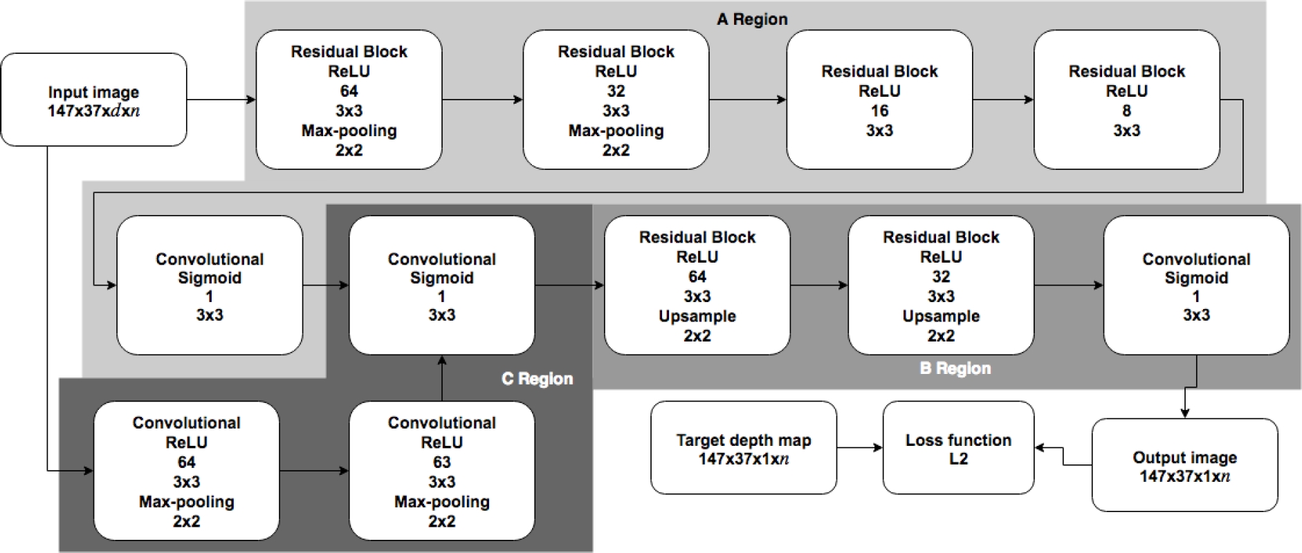
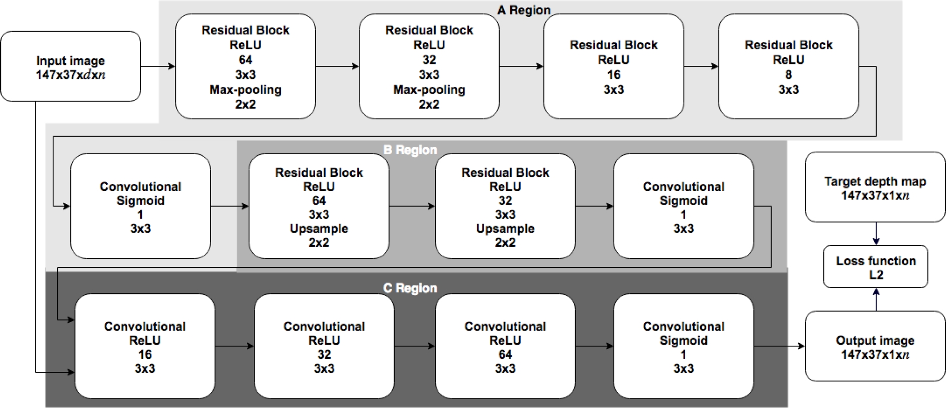
At the end of Region A, we use a convolutional layer with a sigmoid
activation function to limit output limits between 0 and 1. Region B in both
models performs the upsample operation by using two Residual Blocks and a
Convolutional layer, the kernel size in this Region is
As the output of the CNN is smaller than the input image, due to the CNN operations, to recover the original size of the input image, we use Bilinear Interpolation [10], after the last convolutional layer. It is to mention that we describe our models as multi-stage models, but we considered them single-stage models because we only trained them once, we do not train each stage separately as [7] and [6], also we do not apply pre-processing to the input images. The output of all the CNN models are normalized between values of 0 and 1, to optimize the learning of them according to [12], then the images can be converted to grayscale values.
3.3 Loss Function
To train our CNN model we have to minimize an objective loss function. This loss function measures the global error between the target image and the depth reconstruction given by the CNN.
We use the
3.4 Error Measures
To evaluate our models we use several error measures commonly used to compare depth reconstruction with the original targets [20, 2].
Root Mean Square Error (RMSE):
Mean Squared Error (MSE):
Absolute Relative Difference (ARD):
Logarithmic Root Mean Square Error (LRMSE):
Logarithmic Root Mean Square Error Scale-Invariant (LRMSE-SI):
Squared Relative Difference (SRD):
RMSE, MSE and ARD tend to represent the global view error in the images, while and LRMSE, LRMSE-SI and SRD are more representative of the local view error.
4 Experiments and Results
In this section we describe the results of our models. We experimented with two different datasets: KITTY and NYU.
4.1 KITTI Dataset
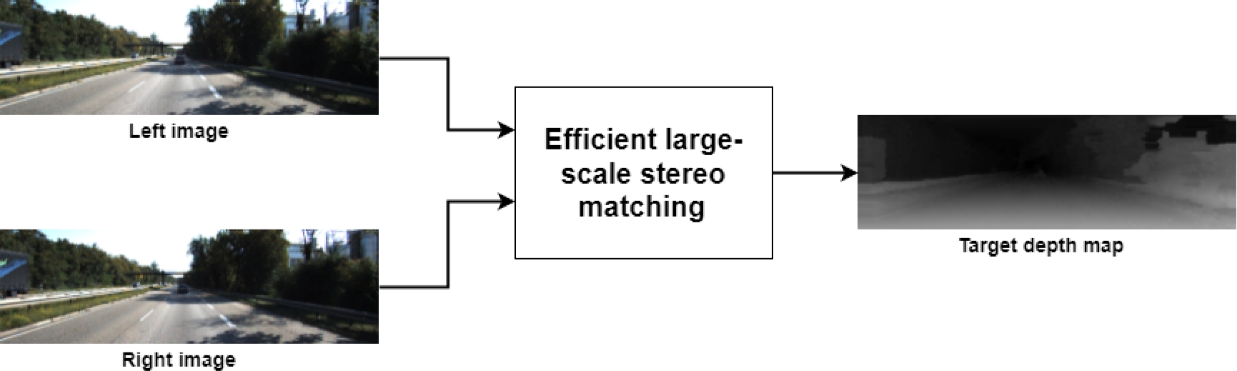
We used the object tracking section of The KITTI Vision Benchmark Suite [8]. This dataset contains 15,000 outdoor scenes given as stereoscopic images. This dataset does not directly contain the target depth maps, so we had to reconstruct the target depth maps using different algorithms such as Semiglobal stereo matching [13] and Blockmatching stereo algorithm [15]. In Fig. 10 an image sample to compare different stereo matching algorithms to obtain the target depth map is shown. Finally, we decided to use the Efficient large-scale stereo matching [9] due to its quality and its evaluation reported in [22]. This algorithm receives a pair of stereo images and its result is the target depth map (see Fig. 11).
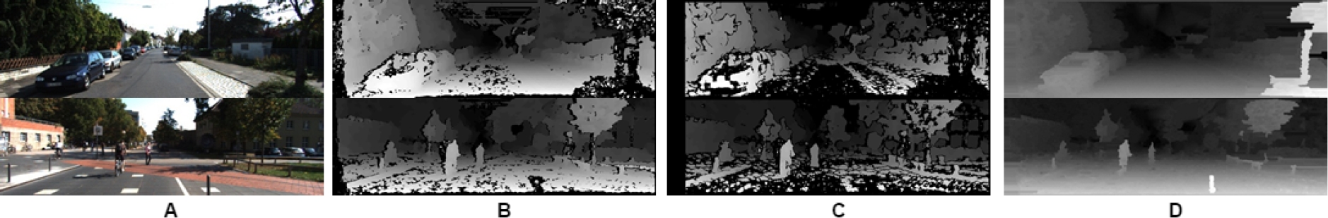
Fig. 10 Target depth map comparison with different stereo matching methods, (A) Stereoscopic images, (B) Semiglobal Matching, (C) Blockmatching method, (D) Large-Scale matching method
We trained our models with Backpropagation [18] and Stochastic Gradient Descent [17]. We used 1,000 iterations and a batch size of 40.
From the dataset we used 12,482 images (left eye) and its
respective target depth map for training, and 2,518 images for testing. Both
input and output images have a size of
We implemented our models with the Python toolbox, Tensorflow [1] which can be trained on a GPU for swift performance. We trained our models on a GPU NVIDIA GTX 1080; it took approximately two days for training and less than a second for testing a single image. As explained in Section 2, for comparison we implemented the model proposed by [2].
This model can be trained with the L2 norm and still obtain better results than the rest of related work. Figure 12 shows a sample of results of our implementation AH of [2], and our proposed models C, SC, SCRX, SCRXU and SCRDU.

Qualitatively comparing results shown in previous figures, it can be seen that our models are capable of reconstructing depth at global view, with slightly better attention to details in local view than previous proposals. For global view we refer to the image in general avoiding small details and for local view we refer to small details such as cars, pedestrians, etc. For a quantitative analysis, Table 1 presents the error measures of all our models and the reimplemented model. RMSE, MSE and ARD measure the global view error in the images, while and LRMSE, LRMSE-SI and SRD measure the local view error.
Table 1 Comparison of error measures between our approach and AH [2] (smaller is better)
| Error | AH | C | SC | SCRX | SCRXU | SCRDU |
| RMSE | 0.1496 | 0.1301 | 0.1082 | 0.1051 | 0.1218 | 0.1348 |
| MSE | 0.0260 | 0.0193 | 0.0132 | 0.0124 | 0.0166 | 0.0213 |
| ARD | 0.4540 | 0.5858 | 0.4813 | 0.4625 | 0.4661 | 0.4350 |
| LRMSE | 0.3377 | 0.3618 | 0.3048 | 0.3081 | 0.3239 | 0.3260 |
| LRMSE-SI | 0.2068 | 0.2269 | 0.1816 | 0.1820 | 0.1980 | 0.1931 |
| SRD | 0.9865 | 1.1982 | 0.8678 | 0.8016 | 0.9528 | 0.9303 |
Comparing our methods with the state of the art, we obtain better results with most of our models, being SCRX Model better at global view while SC Model performs better at local view.
4.2 Improved SCRX Model
While previous models were tested with images of
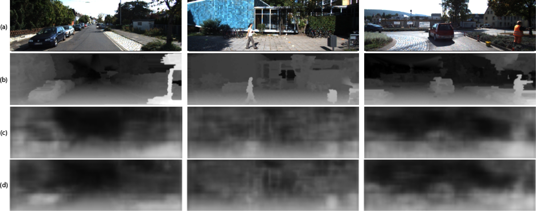
Fig. 13 Sample output of improved SCRX Model. (a) Input image; (b) Target depth map; (c) Output for grayscale input; (d) Output for color input
4.3 Tests on the NYU Dataset
The NYU v2 dataset [24] consists
of 1,449 images of indoor scenes, from which 795 are used for training and 654
for test (the standard training-test split provided with the dataset). Images
were resized to

Fig. 14 Sample output of the improved SCRX Model on the NYU dataset. (a) Input image; (b) Target depth map; (c) Output for grayscale input; (d) Output for color input
As with the previous dataset (KITTI), better results were achieved by using color images (See Table 3). Quantitatively, our model performs better than the prior work as shown in Table 4, the main difference between the results of our model is that we use all the pixels from the target depth map of the dataset, avoiding the cases of invalid pixels.
Table 3 Results of improved SCRX model on the NYU dataset
| Grayscale | Color | |
| RMSE | 0.2138 | 0.2117 |
| MSE | 0.0478 | 0.0473 |
| ARD | 0.0334 | 0.0205 |
| LRMSE | 0.3181 | 0.2915 |
| LRMSE-SI | 0.2376 | 0.2225 |
| SRD | 1.3493 | 0.7574 |
Table 4 Comparison between the state of the art and our proposal on the NYU dataset (smaller is better)
| Authors | RMSE | ARD | LRMSE | |
| Ours | Grayscale Color |
0.2138 0.2117 |
0.0334 0.0205 |
0.3181 0.2915 |
| Liu et al., 2014 | DC-CRF | 1.0600 | 0.3350 | 0.1270 |
| Eigen et al., 2014 | 0.8770 | 0.2140 | 0.2830 | |
| Eigen et al., 2015 | 0.6410 | 0.1580 | 0.2140 | |
| Baig et al., 2016 | GCL | 0.8156 | 0.2523 | 0.0973 |
| RCL | 0.8025 | 0.2415 | 0.0960 | |
| Mousavian et al., 2016 | 0.8160 | 0.2000 | 0.3140 | |
| Lee et al., 2018 | 0.5720 | 0.1320 | 0.1930 |
5 Conclusions and Future work
We have presented five CNN models that require only a single-stage training and perform refinement in the same stage. We tested our models with an existing dataset of stereoscopic images and compared their performance with the state of the art in depth reconstruction.
We found that the use of a residual block instead of convolutional layers improves results.
Using upsample layers improves quantitative results as well, although this may not be directly attested in some cases when examining results qualitatively – some objects appear to be blurred and less defined because of this layer. Using bilinear interpolation instead of upsampling layers improves results. Perspective of the image takes an important role on the reconstruction of depth. Quantitatively, local depth can be estimated with our models, but there is still room for improvement. As a future work we plan to experiment with different kernel sizes, different loss functions and activation functions to further improve our proposed models.

