1 Introduction

This paper analyzes the path not for a non-linear system but for a network of nonlinear systems coupled with delay, which are forced to follow a reference signal generated by a non-linear chaotic system. The control law that guarantees trajectory tracking is obtained using the Lyapunoc-Krasovskii methodology and the PID control law. The control law that guarantees trajectory tracking is obtained by using the Lyapunov methodology and the Fractional Order PID Control Law. It is interesting to note that more than half of the industrial controllers in use today are PID controllers or modified PID controllers. The proportional action tends to stabilize the system, while the integral control action tends to eliminate or reduce steady-state error in response to various inputs.

Derivative control action, when added to a proportional controller, provides a means of obtaining a controller with high sensitivity. An advantage of using derivative control action is that it responds to the rate of change of the actuating error and can produce a significant correction before the magnitude of the actuating error becomes too large.

Derivative control thus anticipates the actuating error, initiates an early corrective action, and tends to increase the stability of the system. The combination of proportional control action, integral control action, and derivative control action is termed proportional-plus-integral-plus-derivative control action. It has the advantages of each of the three individual control actions.

A Fractional Order PID controller, also known as a PIλDα controller, takes on the form ^[1]:

where λ and α are the fractional orders of the controller and e(t) is the system error. Note that the system error e(t) replaces the general function f(t).

The analysis and control of complex behavior in complex networks, which consist of dynamical nodes, has become a point of great interest in recent studies ^[2,3,4]. The complexity in networks comes from their structure and dynamics but also from their topology, which often affects their function.

Recurrent neural networks have been widely used in the fields of optimization, pattern recognition, signal processing and control systems, among others. They have to be designed in such a way that there is one equilibrium point that is globally asymptotically stable.

Trajectory tracking is a very interesting problem in the field of theory of systems control; it allows the implementation of important tasks for automatic control such as: high speed target recognition and tracking, real-time visual inspection, and recognition of context sensitive and moving scenes, among others. We present the results of the design of a control law that guarantees the tracking of general fractional order complex dynamical networks.

2 Mathematical Models

3 Trajectory Tracking

The objective is to develop a control law such that the ith fractional delayed neural network (2) tracks the trajectory of the ith fractional dynamical system (1). We define the tracking error as e_i = x_in - x_i, i = 1, 2, …, N whose time derivative is:

From (1, 2, 3), we obtain:

Adding and subtracting, Winσxit-τ,αit, i=1,2,…,N, to (4), where α_i is defined below, and considering that x_in = e_i + x_i, i = 1,2,..., N, then:

In order to guarantee that the ith neural network (2) tracks the ith reference trajectory (1), the following assumption has to be satisfed:

Assumption 1. There exist functions ρ_i(t) and α_i(t), i = 1, 2, …, N, such that:

Let's us define:

From (6, 7), equation (5) is reduced to:

We can also write:

where we used that c_injn = c_ij and a_injn = a_ij.

Then, with the above equation, equation (8) becomes:

It is clear that e_i = 0, i = 1,2,..., N is an equilibrium point of (10), when u~in=0,i=1,2,…,N . Therefore, the tracking problem can be restated as a global asymptotic stabilization problem for the system (10).

4 Tracking Error Stabilization and Control Design

In order to establish the convergence of (10) to e_i = 0, i = 1, 2, …, N, which ensures the desired tracking, first, we propose the following candidate Lyapunov-Krasovskii function ^[7]:

In fractional calculus, the product rule for the derivative is no longer valid. However, we still have an upper bound for the product that appears in (11). Specifically, from Lemma 1 in ^[8] the time derivative of (11), along the trajectories of (10), and adding the Derivative "D":

If a=1+Kd,α=λ, and wi=KiaDt-αeit, then aDtαwi=Kiet,^[9]

We can then write:

Next, let's consider the following inequality, proved in ^[10,11]:

which holds for all matrices X,Y∈Rn×k and Λ∈Rn×n with Λ=Λ⊺>0. Applying (14) with Λ=In×n to the term ei⊺Winϕσei,xi,i=1,2,…,N, we get:

Since ϕ_σ is Lipschitz, then:

with Lipschitz constant Lϕσi. Applying (16) to 12ϕσ⊺ei,xiWin⊺Winϕσei,xi we obtain:

Next, (15) is reduced to:

Then, we have that:

We define u~ni=u~~i+u~~ij+Kpiei+wi-γ21+Lϕσi2Win2,1,2,…,N, and from (19) we get:

Here we select a+ki=0, so, Kd=-Ki-1;Kd≥0, then Ki≥-1. With this selection of parameters (20) is reduced to:

In this part, if λni-Kp>0,a>0, then aDtαV<0,∀ei,wi,Wni, the traking error is asymptotically stable and it converges to zero for every ei≠0; i.e. the Neural Network will follow the plant asymptotically.

Now, we propose to use the following control law:

^. In this case, VNαe<0,∀e≠0. This means that the proposed control law (21) can globally and asymptotically stabilize the ith error system (10), therefore ensuring the tracking of (1 by 2).

Finally, the control action of the recurrent neural networks is given by:

5 Simulations

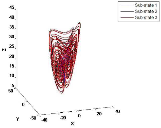
In order to illustrate the applicability of the discussed results, we consider a fractional order dynamical network with just one fractional order Lorenz's node and three identical fractional order Chen's nodes. The single fractional order Lorenz system is described by:

and the Chen's oscillator is described by:

If the system parameters are selected as p₁ = 35, p₂ = 3, p₃ = 28, then the fractional order Lorenz's system and the fractional order Chen's system are shown in Fig. 1 and Fig.2, with α = λ = 1, Fig. 3 and Fig.4, with α = λ = 0.0005 respectively. In this set of system parameters, one unstable equilibrium point of the oscillator (25) is x = (7:9373; 7:9373; 21)T ^[12].

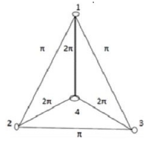
Suppose that each pair of two connected fractional order Lorenz and the fractional order Chen's oscillators are linked together through their identical sub-state variables, i.e.,Γ = diag(1,1,1), and the coupling strengths are c₁₂ = c₂₁ = π, c₂₃ = c₃₂ = π, c₁₃ = c₃₁ = π, c₁₄ = c₄₁ = 2π, c₂₄ = c₄₂ = 2π, c₃₄ = c₄₃ = 2π. Fig. 5 visualizes this entire fractional order dynamical network.

The neural network was selected as:

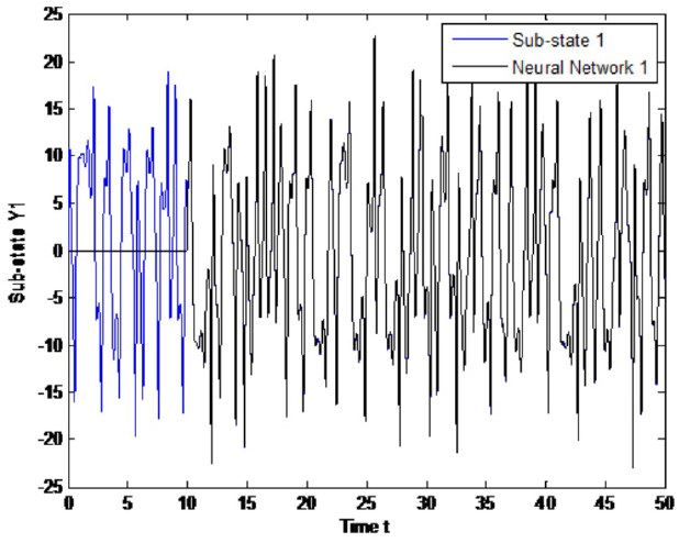
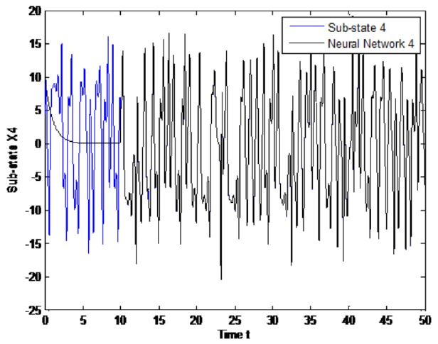
The experiment is performed as follows. Both systems, the recurrent neural network (2) and the dynamical networks (24) and (25), evolve independently; at that time t = 10 Seconds, the proposed control law (22) is incepted. Simulation results are presented in Figs. 6-8, with α = λ = 1, , for sub-sates of node 1. As can be seen, tracking is successfully achieved and error is asymptotically stable, as it is shown in Figs. 9-11, with α = λ = 0.0005 for sub-states of node.

6 Conclusions

We have presented a controller design for trajectory tracking of a fractional general complex dynamical networks. This framework is based on controlling dynamic neural networks using Lyapunov-Krasovskiitheory in the fractional case. We obtained a control law in a purely theoretical way, and can be therefore to a wide range of problems in trajectory tracking.

The proposed control law guarantees the stability of the tracking error between plant and reference signals. The analytical results obtained that predict the stability of the tracking error between plant and reference signals are satisfactory, which can be seen through simulation, these clearly show the desired tracking.

As an example, the proposed control is applied to a simple network with four different nodes and five non-uniform links. In future work, we will consider the stochastic case in fractional systems.