


 text new page (beta)
 English (pdf)
 Article in xml format
 Article references
 Send this article by e-mail
 Cited by SciELO
  Similars in
SciELO
Similars in
SciELO 
 Permalink
1 Introduction
Image segmentation is an important task in the fields of image processing and computer vision. Segmentation is a process of dividing an image into different regions such that each region is nearly homogeneous, whereas the union of any two regions is not. The level to which the division is carried depends on the problem being solved. That is, segmentation should stop when the objects of interest in an application have been isolated. Image segmentation algorithms generally are based on one of two basic properties of intensity values: discontinuity and similarity. In the first category, the approach is to partition an image based on abrupt changes in intensity, such as edges in an image. The principal approaches in the second category are based on partitioning an image into regions that are similar according to a set of predefined criteria [1].
The main objective of image segmentation is to find objects or regions with the same features or attributes of pixels, as could be grey levels, textures, or colors. Several segmentation methods have been developed to do this task, such as edge detection, region growth, histogram thresholding, clustering, etc. [2-7]. The low level processing refers to a representation of the image in pixel or a small group of pixels and one of the most common and widely used tasks for this level is clustering [8]. According to the above, in this paper we use a hybrid clustering method based on clustering algorithms, specifically the Possibilistic Fuzzy c-Means (PFCM), which was proposed in [9].
Cluster analysis is an unsupervised data analysis task, trying to group data objects into clusters, such that similar data objects are assigned to the same cluster whereas dissimilar data objects should belong to different clusters [10]. In that sense, clustering algorithms are used to find groups in unlabeled data, mainly based on a similarity measure between the data patterns and the prototypes. This means that similar patterns are placed together in the same cluster. So, in the case of image segmentation, the identification of regions is based fundamentally on the distribution of pixel attributes in the feature space, and does not take into consideration the spatial distribution of pixels in an image. This way each pixel pattern is assigned to the region with the nearest or most similar prototype according to the features took into account. Thus, this process forcedly distribute every pixel patterns to the different regions, even if some pixels are not very representative of the region as a whole.
For this reason, in many cases it is not sufficient to identify the regions or objects of an image, but to distinguish, through the variations in intensity, the imperfections or marked differences present in the objects or regions. These imperfections are considered here as atypical pixels, which are very common to find in the different objects or regions of an image. For the three cases considered in this work these imperfections could be the result of a light reflection over an object but, and this is a very interesting case, they could be real imperfect features that can be used aid in image analysis, e.g in medical diagnosis or industrial quality evaluations.
Atypical pixels of an object or a region are generally difficult to detect because they represent a minority among the total pixels of each particular cluster in the image. Besides, the traditional process to increase the number of regions to identify through clustering algorithms, can force to use a great quantity of regions in order to detect the atypical pixels within the image, increasing the computational cost, and the possibilities to fall into a local minimum or a saddle point. A different and new approach, as proposed in this work, is to find the main regions in the image and latter, inside them, to find sub-regions corresponding to typical and atypical pixels for each previous identified region. The main purpose is to find imperfections generally represented by the pixels that have the minimal values of the features belonging to each region.
In a variety of applications based on images analysis to detect the zones of highest interest, such as cancer risk analysis, the less typical pixels, representing a tissue with particular characteristics, or that tend to fall outside of a normal pattern, are precisely the most interesting because they represent a variation with respect to normal pixels or to healthy tissue in the case of cancer risk analysis. We therefore propose image sub-segmentation as an alternative to identify this kind of pixels after an image is segmented in an acceptable way.
For the image sub-segmentation we propose using the PFCM clustering algorithm, as it provides fuzzy membership μik and possibilistic membership or typicality values tik for every pattern of the data set [9]. Therefore, we get a more informed segmentation about the membership of the pixels to each one of the regions. For the three cases of applications presented in this work, the images are represented in gray levels and this is the only feature used here.
The purpose of this work is to find sub-regions using the advantages offered by the PFCM clustering algorithm, which has the qualities of both the Fuzzy c-Means (FCM) [11] and the Possibilistic c-Means (PCM) [12]. The c-partition generated by FCM help us to create Fuzzy Regions (FR), whereas the partition generated by PCM helps us to identify Possibility Regions (PR), and both (FR and PR) the sub-regions, corresponding to the typical and atypical pixels respectively. We use the typicality values tik to divide each PR Si, i... c, in two sub-regions: the sub-region of typical pixels, or pixels with typicality values greater or equal to a specified threshold α, and the sub-region with atypical pixels, or pixels with typicality values below the established threshold α.
The rest of this paper is organized as follows. Section 2 presents the fundamental concepts of image segmentation, Section 3 describes the theory of the clustering algorithms (FCM, PCM and PFCM). Section 4 presents the approach of the sub-segmentation based in PFCM as well as how to use the membership μik and typicality tik values for image sub-segmentation. Section 5 presents the results with images of three kinds of applications. Finally, Section 6 gives the main conclusions of this work.
2 Image Segmentation
Image segmentation is a challenge in image analysis due to that the segmentation result plays an important role in further image processing [5]. The aim of the segmentation is to divide an image into several non-overlapping meaningful regions with homogeneous characteristics extracted of the pixels. On other words, segmentation is basically clustering of the pixels in the image according to some criteria.
If I(x,y), x ∈ X and y ∈ Y, represents the whole image where we try to identify regions and their typical and atypical pixels. The segmentation is a process that partitions I(x,y) in several regions S1(x,y), S2(x,y),…, Sc(x,y), such that the following conditions are desirable:
In the first condition it is assumed that the union of the segmented regions, Si, i=1,...,c, allows to build the complete image, whereas in the second condition it is assumed that the image is partitioned into a set of non-overlapping or disjoint regions.
In other words, it is desirable to identify all the objects in an image and that they would be clearly differentiated among them.
Nowadays, there exists many methods for image segmentation based on different principles. In this work, we use a hybrid clustering algorithm (PFCM) derived from the family of c-Means methods and described in the next section. This approach has been selected as it is founded on membership μik and typicality tik values, such that each pixel is evaluated against all the prototypes and the most similar prototype. Therefore, that facilitates the association of the pixels with the most representative regions that partition the whole image. Clustering is commonly used for segmentation, as there exists a great similarity between them. In fact, the main difference is that clustering was developed for feature spaces, whereas image segmentation was developed for the spatial domain of the image.
As was mentioned in the introduction of this work, we only use the gray intensity level as feature. Therefore, a one-dimensional vector is built with a mapping from the original space of the image to gray levels of the pixels, as follows:
where
2.1 Image Segmentation by Partitional Clustering Algorithms
The partitional clustering algorithms are one most popular unsupervised pattern classification techniques used for the partition a set of objects into k groups. According to that characteristic, the partitional clustering algorithms are an excellent option to perform the image segmentation task. The partitional clustering algorithms has been successfully used for feature analysis, clustering, and classifier design in a variety of scientific disciplines such as astronomy, geology, medical imaging, target recognition and image segmentation. These algorithms find more or less homogeneous groups by iteratively minimizing a cost function from the similarity among the pixels and the prototypes in the features space.
The partitional clustering algorithm most used for image segmentation is the FCM [13-17].
An image is represented in an n-dimensional space that depends on the number of features or attributes associated to the pixels, where each point in this space will be named pixel or pattern.
Generally, an image is defined in a rectangular lattice where each pixel has its particular position; even though an image is pre-processed to reduce the level of noise or to improve the contrast, the lattice has no changes.
As previously mentioned, the segmentation by clustering algorithms is normally based on the values of the features or attributes of the pixels, and the spatial distribution is seldom taken into account.
Thus, the results are very sensitive to noise, and this can produce regions with holes (pixels that belong to other regions) in the spatial domain of the image. That means that there could be a lack of spatial homogeneity in the regions. Nowadays there exist some partitional clustering algorithms that include spatial information through the objective function [5], [18-21]. However, in this work only the gray level of each pixel is considered for the features.
3 Clustering Algorithms
In this work we take advantage of the qualities of fuzzy and possibilistic clustering algorithms in order to find c groups in a set of unlabeled data set Z={z1, z2,...,zk,..., zn}, c < N, in an m-dimensional space, where each data zk is associated with the nearest prototype, or group center, vi among the c possible groups (z = 1, ... , c).
The membership of each data zk to the different groups depends on the kind of partition of the m-dimensional space where the data set is defined. This way, a c-partition can be either: hard, fuzzy, or possibilistic [22].
The hard c-partition of the space for a data set Z={zk | k=1,2,...,N} of finite dimension, where 1<c<N, is defined by eqs. (3), (4) defines the fuzzy c-partition, whereas eq. (5) defines the possibilistic c-partition.
3.1 Fuzzy c-Means Algorithm
The Fuzzy c-Means clustering algorithm (FCM) was initially developed by Dunn [23], and generalized later by Bezdek [11]. This algorithm is based on the optimization of the objective function given by (6):
where the membership matrix
Theorem FCM [11]: If
being (7) and (8) necessary but not sufficient conditions.
Following the previous equations of the FCM algorithm, the solution can be reached with the next steps:
Given the data set Z choose the number of clusters 1<c<N, the weighting exponent m>1, as well as the ending tolerance δ>0.
Provide an initial value to each one of the prototypes vi, i=1,..,c. These values are generally given in a random way.
Calculate the distance of each one of the zk to each one of the prototypes vi, using
If
Update the new values of the prototypes vi using (8).
Verify if the error is equal or lower than
If this is truth, stop. Else, go to step 2.
The FCM is an algorithm that calculates a membership value μik for each point zk in function of all prototypes vi. The sum of the membership values of zk to the c groups must be equal to one. However, a problem arises when there are several equidistant points from the prototypes of the groups, because the FCM is not able to detect noise points or nearest and furthest points from the prototypes. Pal et al. [24] show an example with two points located in the boundary of two groups, one point near to the prototypes and the other one far away from them. This must be handled with care, as both points are not equally representative of the groups, even if they have the same membership values. One way to overcome this inconvenience is to use a possibilistic algorithm.
3.2 Possibilistic c-Means Algorithm
The Possibilistic c-Means clustering algorithm (PCM) [12] is based on typicality values and relaxes the constraint of the FCM concerning the sum of membership values of a point to all the c groups, which must be equal to one. Thus, the PCM identifies the similarity of data points with an alone prototype vi using a typicality values that takes values in [0,1]. The nearest data points to the prototypes are considered typical, further data points are atypical and data points with zero, or almost zero, typicality values are considered noise [25]. The objective function Jpcm proposed by Krishnapuram [12] for this algorithm is given by:
where
The first term of Jpcm is similar to that of the FCM objective function, which is based on the distance of the points to the prototypes. The second term, that includes a penalty γi tries to bring the typicality values tik toward 1.
Theorem PCM [12]: If
Being (10) and (11) only necessary but not sufficient conditions.
Krishnapuram and Keller [12] [26] recommend to apply the FCM at a first time, such that the initial values of the PCM algorithm can be estimated.
They also suggest the calculus of the penalty value y with (12):
where K>0, although the most common value is K=1, and the membership values μik are those calculated with the FCM algorithm in order to reduce the influence of noise.
The PCM algorithm is very sensitive to the γi values, and the typicality values depend directly on it. For example, if the value of γi is small, the typicality values tik of T are also small, whereas if the value of γi is high, the tik are also high. For this work, the γi values are obtained using the eq. (12).
In order to avoid a problem with the initial PCM algorithm, as sometimes the prototypes of different groups coincided [27], even if the natural structure of data has well delimited different groups, Tim et al. [28-30] have modified the objective function to include a constraint based on the repulsion among groups, thus avoiding identical groups when they must be different.
The problems of the FCM and PCM clustering algorithms, outlier sensitivity for the FCM and the coincident clusters for the PCM, as it has been explained before, have been solved in the hybrid algorithm PFCM that is described in the next subsection, and it is an excellent candidate for image sub-segmentation.
3.3 PFCM Clustering Algorithm
Pal et al. [31] have proposed to use the membership values as well as the typicality values, looking for a better clustering algorithm, and they called it Fuzzy Possibilistic c-Means (FPCM). However, the sum equal to one of the typicality values for each point was the origin of a problem, particularly when the algorithm uses a lot of data.
In order to avoid this problem, Pal et al. [9] proposed to relax this constraint and they developed the PFCM clustering algorithm, where the function to be optimized is given by (13):
and subject to the constraints
Theorem PFCM [9]: If
being (14), (15), and (16) only necessary but not sufficient conditions.
The iterative process of this algorithm follows the next steps:
Given the data set Z choose the number of clusters 1<c<N, the weighting exponents m>1, η>1, and the values of the constants a>0, and b>0.
Provide an initial value to each one of the prototypes vi, i=1,.., c. These values are generally given in a random way.
Run the FCM algorithm as described in Section 3.1.
With these results and (12) calculate the penalty parameter γi for each cluster i. Take K=1.
Calculate the distance of Zk to each one of the prototypes vi using
If
If
Update the value of the prototypes vi using (16).
Verify if the error is equal or lower than
Using both membership and typicality values, it is possible to identify groups and theirs most or least representative data as well. We therefore use them to create the sub-groups of typical and atypical data for each group.
4 Image Sub-segmentation with the PFCM algorithm
In a previous work [32] we have made an analogy between the theory of prototypes proposed by Rosch [33], and clustering algorithms based on fuzzy and possibilistic concepts. There, we analyze the concept of typicality in the context of the theory of prototypes, where prototypes are the most typical examples, according to a given criterion, to represent groups, and they have the most important features of the corresponding group.
In the case of birds, for example, the dove is more typical than the ostrich and the penguin, because it has more features of a bird. However, ostriches and penguins are members of the category of birds, and different from horses and cows to cite an example. Therefore, there is an internal resemblance among the members of a group, and an external dissimilarity to the members of other categories, even when several categories share some features, as it happens with birds and reptiles, as both kinds of animals reproduce by eggs. However, each group has its own features that define them as members of a particular group, and different to the others. A similar situation happens with a numerical data set, that is, it is possible to take into account an external dissimilarity (FCM) and an internal resemblance (PCM) among patterns and prototypes.
In this way, we can apply a hybrid clustering algorithm, as the PFCM, such that the external dissimilarity and the internal resemblance can be represented by membership values jik and typicality values tk respectively, as a possibility to identify typical and atypical pixels into each identified region in the whole space of the image. This is a good option to find more information directly related with the pixels of an image, as for the three cases considered in this work, where the most typical or the most atypical data can be easily identified inside the regions provided by the hybrid algorithm.
For example, select a threshold a, 0<α<1, such that pixels in each region in one image can be divided in two sub-regions, each one containing typical or atypical pixels, where the typical pixels have the greatest typicality values. So, with a high value of α we can find the most typical pixels of a region, and with a low value we find the most atypical pixels. In this work, the threshold must be the best compromise to separate correctly the atypical pixels from the typical ones.
The FCM algorithm is among the most popular partitional clustering algorithms. However, and due to the constraint on the sum of the membership values of a point to all the groups must be one, the membership of a point to a particular group depends on the membership to other groups. So, the membership value can be interpreted as a relative typicality, considering that in the Zadeh's formulation of fuzzy set theory [34], the membership value of a point in the universe of discourse to a fuzzy set does not depend on the membership values to other fuzzy sets [35]. On the other hand, the PCM algorithm provides typicality values that can be interpreted as an absolute typicality, because this value only depends on the similarity between a point and a prototype. This difference between relative and absolute typicality allows us to identify typical and atypical pixels in each one of the identified regions in the image.
Next, we describe the proposed approach for the sub-segmentation of images using hybrid algorithms as the PFCM.
Proposed approach for the sub-segmentation of images with the PFCM clustering algorithm is as follows.
Get the vector of features through the mapping of the original image.
Assign a value to the parameters (a, b, m, η) as well as to the number of clusters c, or number of regions Si, i = 1,…, c, to partition the space of features of the image.
-
Run the PFCM algorithm to get:
The steps to run the algorithm has been described in Section 3.3.
-
Label each pixel Zk, k=1,..., N, according to the FR with maximum membership value in
such that each pixel zk can only belong to one region Si.
-
Label each pixel zk, k=1,... , N, according to the PR with maximum typicality value in
such that each pixel zk can only belong to one region Si.
-
Get the maximum typicality value for each point from the previous Si matrix and put it in the Tmax matrix:
Select a value for the threshold α.
-
With α and the Tmax matrix, separate all the pixels in two sub-matrices (T1,T2), the first matrix:
which contains the typical pixels, and second matrix:
containing the atypical pixels.
-
From the labeled pixels zk of the T1 sub-matrix the following sub-regions can be generated:
and from the T2 sub-matrix:
such that each PR is defined by:
Select the sub-matrix T1 or T2 of interest for the corresponding analysis.
Fig. 1 shows the process of the proposed approach for the image sub-segmentation applying the PFCM.

5 Experimental Results
The proposed approach has been applied in three different domain of applications. Here we use four images to show the results: a drop of milk, ROI images of digitized mammograms [36] and a board of wood [37]; seeing these images is evident why the atypical pixels are of great interest. The parameters (a, b, m and η) of the PFCM clustering algorithm have a great influence on the results. The values of a and b represent a relative importance of membership and typicality in the computation of prototypes. If the value of a is greater than the value of b, the prototypes calculated with eq. (16) are more influenced by the membership values. Conversely, if b is greater than a the typicality values have more influence, and hence the prototypes are expected to be less affected by noise. So, in order to reduce the effect of the outlier pixels and to find prototypes that depend more on the most representative pixels of each regions, a higher value of b than a must be used, as proposed by Pal et al. [9]. From here, the values used for these parameters are: a=1 and b=2. On the other hand, the parameters m=2 and η=2 represent an absolute weight of membership values μik and typicality values tik, respectively. As μik and tik take values in [0, 1], values of m and η greater than 1, as defined for the algorithm, reduce the effect of membership and typicality values. This suggest that low values must be taken for both parameters. In fact, it is characteristic to use m=2 for the FCM algorithm and those derived from it. As we want to weight the typicality values in a similar way we have selected η=2.
5.1 Sub-Segmentation of the Drop of Milk Image
The image of the drop of milk is very simple as there are only two easily identifiable regions: the drop of milk and the background. However, some pixels in both regions differ significantly from the rest of pixels, and they are considered as atypical. In this case, the great difference of gray level of some pixels results from the illumination of the scene and the shape of the object. These pixels can be identified applying the methodology for the sub-segmentation of images presented in Section 4, as follows.
Once the values of parameters of the PFCM clustering algorithm have been defined, it can be applied in order to segment and afterwards to subsegment the image in different regions or groups, and sub-regions or sub-groups, respectively. The estimated values of the prototypes for the drop of milk image are v 1= 187.6164 and v2= 49.0242 with the following parameters of the PFCM, a=1, b=2, m=2 and η = 2. As can be seen in eq. (16), these ones depend on the membership and typicality values.
When the values of the U and T matrices of the
PFCM clustering algorithm are available, we can build the groups using the
membership values of
Fig. 2 shows the original image to process
and different results. Fig. 2(a) contains
the original image of the drop of milk. Fig.
2(b) the identified FR with the membership values of
U in two regions FR: (S1 and
S2), and Fig. 2(d) the two PR
(S1, S2) and four
sub-regions S1 :
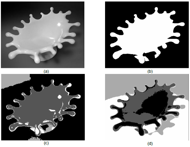
Fig. 2 Comparison of segmentation results for a drop of milk image with 400 x 320 pixels. (a) Original image. Segmentation with the PFCM: (b) in two FR with the membership matrix U, (c) in four possibility sub-regions with the typicality matrix T, and (d) in four FR with the FCM
The Fig. 2(c) shows two FR: (S1 and S2). The first one and in white color, S1, represents the drop of milk. The second FR and in black color, S2, represents the background. This result is very similar to that obtained with the FCM alone. It can be considered as a good segmentation between the drop of milk and the background, except for the region in the lower part of the drop of milk, due to the shadow generated by this one, because it has a gray intensity level very close to the value of the prototype (49.0242) for the background.
Fig. 2(c) shows the sub-segmentation
results of the image with the typicality values tik and a threshold
α=0.2, according to the approach previously described. Each PR S1 and
S2 is represented by two sub-regions. The first PR S1
is represented by colors; dark gray for the
In order to get a clearer idea of the subsegmentation, the Figs.: 3(c), 3(d),
3(e) and 3(f) show the PR S1 and S2 respectively with
the original pixels. The Fig. 3(c) and
3(d) contains a sub-segmentation of the
PR S1 or the drop of milk. These pixels are the most typical for a
threshold α=0.2, that is, they are the nearest pixels to the prototype
v1. As can be seen,
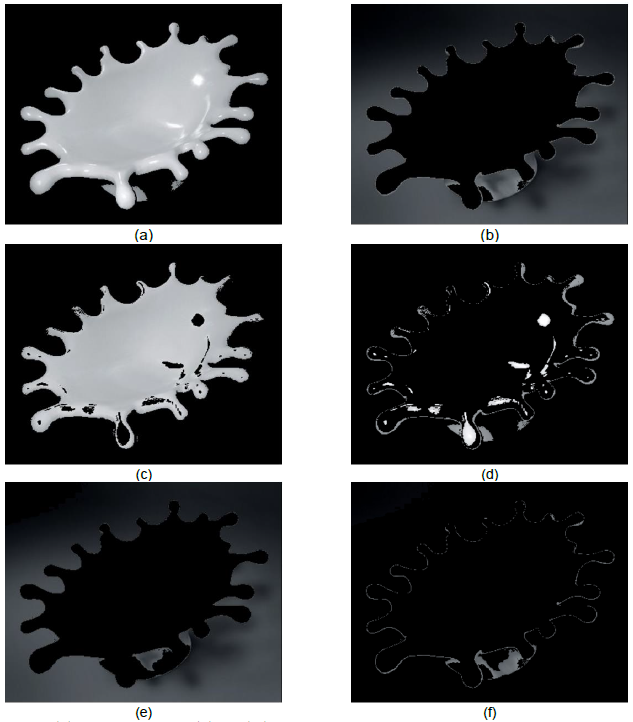
Fig. 3 Segmentation and sub-segmentation with the original pixels and a
black background. (a) FR S1, (b) FR
S2. (c) PR
Therefore, in the image the atypical pixels have two gray levels very different, one near to the white color and the other near to a medium gray level or near to the mean value between the white and black colors, which represents the prototypes (v1 and v2). This is the reason why the atypical pixels, those reflecting the light and those at the boundary, are observed in the Fig. 3(d). Reducing the value of the threshold, in this case α<0.2, allows to identify the most atypical pixels of the PR S1 in the image. The corresponding pixels are those with gray level near to the white color, and the atypical pixels located at the boundary of the drop of milk are not detected this time.
Figs. 3(e) and 3(f) are included to show the sub-segmentation of PR
S2. In the PR
In Fig. 3(d) and Fig. 3(f), show the atypical pixels. These pixels are found
at the end of the prototypes (v1 and
v2). For example, in the sub-region
In the sub-region
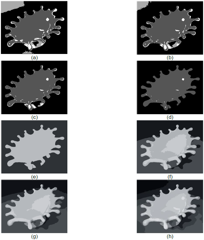
Fig. 4 Value threshold effect α in the sub-segmentation process with PFCM, and segmentation with the FCM in several regions. (a) α = 0.2, (b) α = 0.15, (c) α = 0.1 and (d) α = 0.05. (e) FCM 2 regions, (f) FCM 4 regions, (g) FCM 6 regions and (h) FCM 8 regions
As can be seen in the previous results, the subsegmentation method allows us to find the most representative pixels of each region (according the value of α selected). Nevertheless, in images where there exist a great variation in the values of the features, caused in this particular example by the reflection of the light and the shadow of the drop of milk, it is very difficult to segment totally the object. On the other hand, Fig. 2(d) shows the results of a classical approach for image segmentation corresponding, in this case, to four FR with the FCM. In order to detect the atypical pixels as a sole group, for example those of the S1 region, the number of regions must be increased in a significantly way following a classical approach. In the Figs. 4(e, f, g, h) it has increased the number of regions. The atypical pixels are beginning to see when the image has been segmented into 8 regions.
A comparison between Fig. 2(c) and Fig. 2(d) clearly shows the difficulty and the different results between both approaches, the sub-segmentation method and a classical method, in this case the latter done with the FCM clustering algorithm. With the classical approach more or less homogeneous regions are obtained from the number of regions in which the image is segmented, if required find more atypical pixels must increase the number of regions. For the sub-segmentation, it is necessary to run the algorithm once and use the T matrix and vary the value of a to find the atypical pixels.
5.2 Sub-Segmentation of Digitized Mammograms
Breast cancer is one of the main causes of dead of women around the world. Early detection of breast cancer is essential in reducing life loss. Clusters of Microcalcifications (MCs) are an important early sign of breast cancer. MCs appear as bright spots of calcium deposits. Individual microcalcification is sometimes difficult to detect because of the surrounding breast tissue, their variation in shape, orientation, brightness, and diameter size [38-39]. MCs are potential indicators of malignant types of breast cancer. Therefore, their detection is very important to prevent and treat this disease. However, it is still a hard task to detect all the MCs in mammograms, because of the poor contrast with the tissue that surrounds them.
The approach proposed in Section 4 is now applied to the identification of MCs in two ROI images of digitized mammograms. These kinds of images have the characteristic that the changes in the gray intensity level in the regions of the microcalcifications can difficult this task. As the purpose of this work is to show the advantages of the sub-segmentation method, the ROI images were not pre-processed for the enhancement of features in order to identify the anomalies present in the images, as it is generally done by someone who tries to solve the problem of microcalcification identification.
The two ROI images of digitized mammograms of Fig. 5(a) and Fig. 5(c) are only segmented in two PR, one of them, S1, for the healthy tissue and the other one, S2, for the tissue that differs significantly from the healthy tissue or tissue that contains MCs. The MCs appear in small clusters, with few pixels, with relatively high intensity and closed contours compared with their neighboring pixels. Although the gray intensity level of MCs can vary significantly between healthy and abnormal tissue, MCs have a few quantity of pixels and this makes difficult their identification.
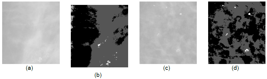
Fig. 5 (a) ROI image of the mammogram A with 256 x 256 pixels, (b) four sub-groups of mammogram A using the typicality matrix T, (c) ROI image of the mammogram B with 256 x 256 pixels, and (d) four sub-groups of mammogram B using the typicality matrix T
Fig. 5(b) and Fig. 5(d) contain the subsegmentation results, where we attempt to
identify the brighter pixels or pixels corresponding to MCs, as these are the
least representative of healthy tissue. Fig.
5(b) shows the results of the Fig.
5(a) with a threshold α=0.1 obtained experimentally. This value was
selected after several tests, and it was considered the best value for this
particular case. The sub-segmentation of Fig.
5(b) is given according to the following colors: the PR
The threshold α for the image of Fig. 5(d) is α=0.02. This value is much smaller than the threshold of image in Fig. 5(b), as there is a more important contrast between healthy tissue and pixels with higher gray intensity levels.
As contrast increases, it makes that the atypical pixels be further from the
prototypes and the algorithm gives them a smaller typicality value. So, a
smaller threshold α value is required. The converse is also true, that means, as
the contrast decreases, the threshold α value must be increased. Therefore, the
best value of this parameter is application dependent. Fig. 5(d) shows the results of the image sub-segmentation of
the Fig. 5(c): the PR
In order to analyze the main differences between the sub-segmentation and the segmentation through a partitional clustering algorithms other experiment is presented.
5.2.1 Image Selection
A set of ten images were selected from several mammograms of the mini-MIAS database provided by the Mammographic Image Analysis Society [36].
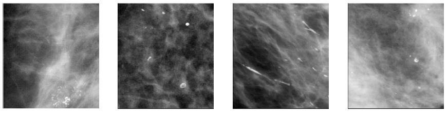
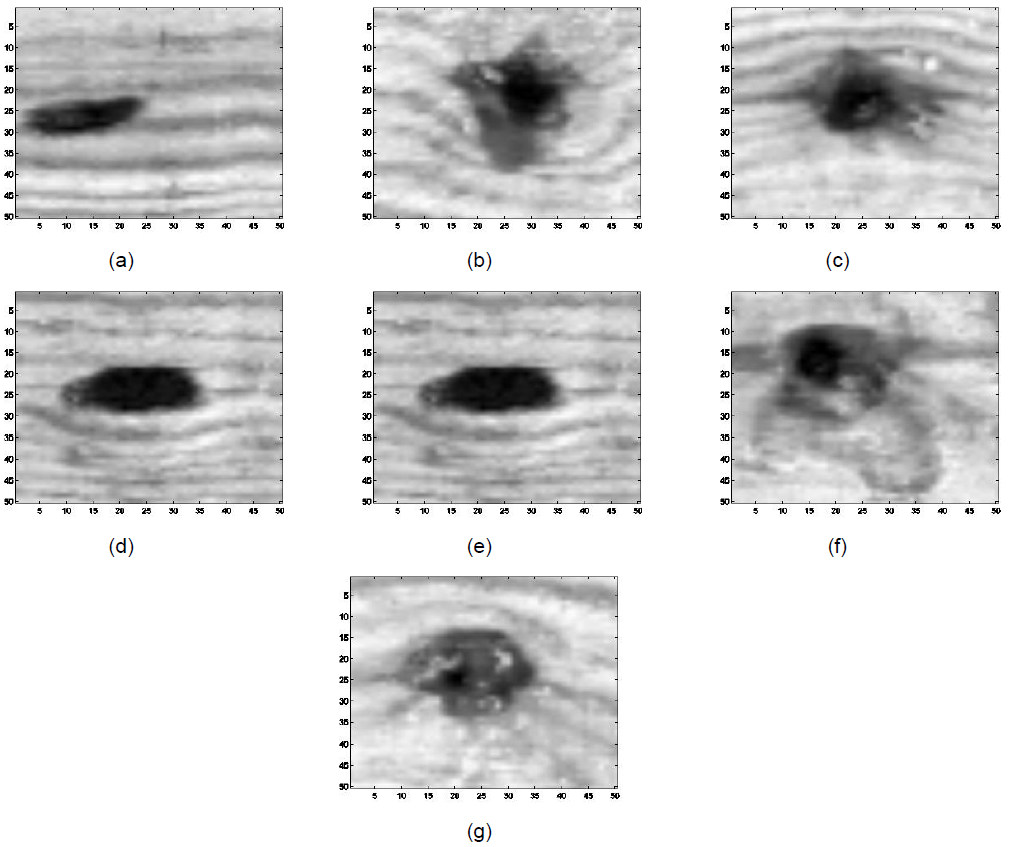
The areas in which abnormalities such as MCs were located were taken as regions of interest (ROI). In this experiment the size of the ROI images are of 256 x 256 pixels with spatial resolution of 200 urn/pixel. Figure 6 shows some ROIs images used in this experiment.
5.2.2 Image Enhancement
With the aim to improve the contrast between the MCs and background in the ROI image, a morphological contrast enhancement technique is used in this experiment. This morphological contrast enhancement is an image enhancement technique based on mathematical morphology operation known as top-hat transforms. This technique was used in previous works such as, [40-44], with satisfactory results in the MCs detection.
The morphological top-hat transform is used to enhance ROI images, with the aim of detecting objects that differ in brightness from the surrounding background; in this case, it was used to increase the contrast between the MCs and the background. The top-hat transform is defined by the following equation:
where, I is the input ROI image, It
is the transformed ROI image, SE is the structuring element,
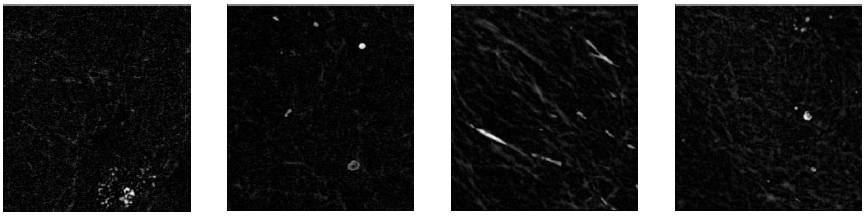
During image enhancement, the same SE at different sizes, 3 x 3, 5 x 5, 7 x 7, was applied to perform the top-hat transform. The SE used in this experiment was a flat disk-shaped. Figure 7 shows the ROI images processed by the top-hat transform with a SE of 7 x 7.
5.2.3 Image Segmentation by Clustering Algorithms
A data vector Z for each ROI is generated for each of the images obtained from the previous stage. Thus, a unidimensional vector xse is built by mapping the images to the pixels as follows:
where se is the size of the SE,
For data vector Z, two proposed clustering techniques are then applied to obtain a label for each pattern belonging to each cluster of the partition of feature space, where only one cluster corresponds to MCs, which generally appear in a group of just a few patterns (pixels), and the remaining clusters correspond to normal (healthy) tissue. The initial conditions and results for each proposed clustering technique are presented below.
5.2.4 MCs Segmentation by FCM
The initial conditions for this approach are as follows: Clusters number: 2 to 5. Prototypes: initialized as random values. Weighting exponent m = 2. Distance measure: Euclidean distance function.
Fig. 8 shows segmented ROI images with different cluster values obtained after applying the FCM (presented in the Subsection 3.1) to Z.
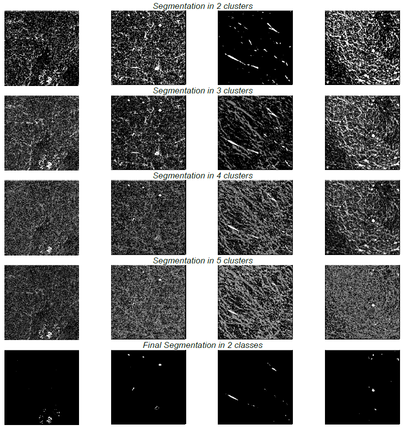
5.2.5 MCs sub-Segmentation by PFCM
In this experiment, the approach presented in Section 4 is applied. The initial conditions are as follows: Clusters number: 2. Prototypes initialized as random values. Distance measure:
Euclidean distance function. Parameters of the PFCM: m = 2, a = 1, b = 2, η = 2. α = [0.03 0.02 0.01]
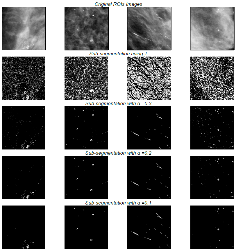
Fig. 9 shows segmented ROI images with different threshold values a obtained after applying the approach presented in Section 4 to the data vector Z.
5.3 Sub-Segmentation for Wood Surface Defect Detection
Every person that uses wood, for construction or ornamental purposes, will be looking material of high quality or free of defects according to establish standards. As everybody knows, the price of a board of wood is directly related to its quality, and this one is characterized by the number of defects, their size and distribution.
A defect is every irregularity that reduces the durability, the resistance, the aesthetic value, or the useful volume of the wood.
In this application we focus on the detection of defects in the surface of the wood, such as knots, the most natural and common problem [45-47].
These defects are classified in seven categories, identified as: Dry defect (DE), Encased defect (EN), Sound defect (SO), Leaf defect (LE), Edge defect (ED), Horn defect (HO), and Defect (DE) [48]. In a manual inspection process, an inspector identifies the defects based on the characteristics of shape, size, structure, and color.
In a common visual inspection, the classification is based on the geometrical characteristics of the knots, such as the size, but also in the size of the smallest square that encloses each knot, the diameter, the position in the wood, and the mean gray level [49]. An automatic inspection process of the wood surface follows the next 5 steps: (1) image acquisition, (2) image segmentation for detection of regions of interest where there are defects or knots on the surface of the wood, (3) features extraction, (4) selection of features, and finally (5) the classification [50]. As this paper is focused on the sub-segmentation of images, this is applied to the step 2, where a board of wood is divided in two regions, the clean wood and wood with defects.
In this particular application, the objective of the sub-segmentation of the image of a board of wood is to identify defects (knots) in lumber boards in order to evaluate its quality. As can be seen in Fig. 10(a), the appearance of sawn timber has huge natural variations, and shape of knots are very different from wood and they can be easily identified by a human inspector. However, for automatic wood inspection systems these variations are a major source for complication.
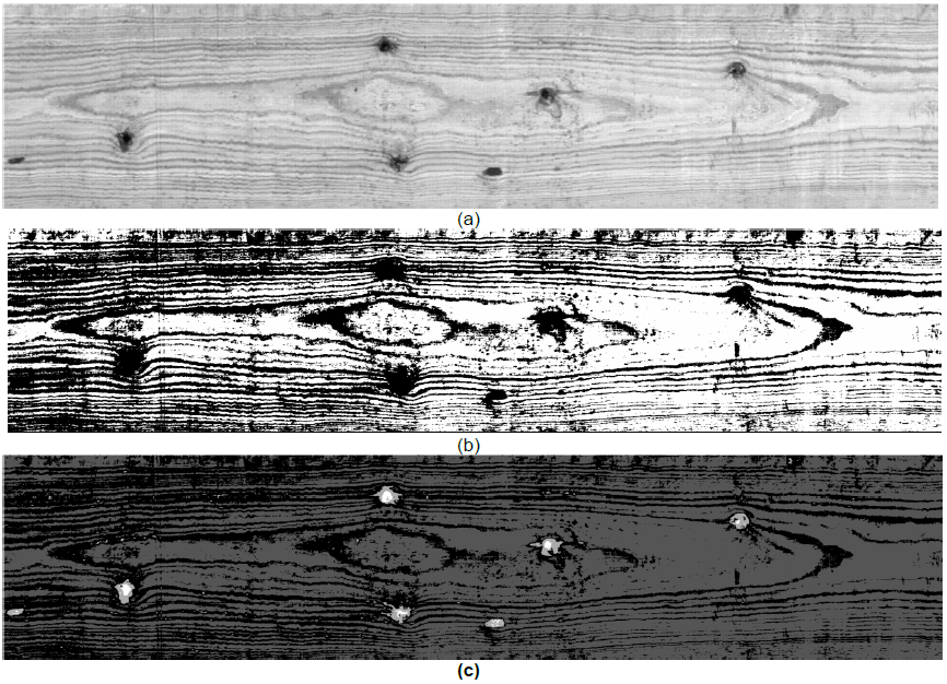
Fig. 10 (a) Original image of a board of wood with several knots and resolution of 523 x 2406 pixels, (b) segmentation of the image in two groups with the membership matrix U, (c) sub-segmentation of the image in four sub-groups with the typicality matrix T
Fig. 10(b) shows the results of the FR segmentation, where the features of the wood are divided in an acceptable way. The estimated values of the Table are v1=178.4531 and v2= 205.1826, with the following parameters of the PFCM, a =1, b =2, m =2, η =2. Fig. 10(c) shows the results of segmentation of the wood surface into two PR S1 and S2, the first region is represented in black color and the second one in white. As can be seen, the knots are within group S1. This is a consequence of the constraint on the sum of membership values μik of a given pixel Zk that must be equal to one for all groups. Therefore, to find the knots with the membership values μk only, we need to increase the number of groups Si in a significant way, and this number is application dependent as the gray intensity level varies significantly from one board to another.
Processing the image as proposed in the previous section provides a segmentation
in two groups, which, at once, are divided in order to identify the typical and
atypical pixels of each group. The first group S1 is
formed by the subgroups
6 Conclusions
In this work, we have proposed to take profit of the membership and typicality values for the subsegmentation of images, as an easy way to identify atypical pixels. The main problem for this is that atypical pixels are present in a few quantity. However, they could be related to quality, so they are of great interest in a wide field of applications, as in the last two cases considered in this document.
Three cases have been considered here: a drop of milk, ROI images extracted from mammograms, and a board of wood. In the first case, it was shown the interest of the proposed approach relative to a classical approach of image segmentation. In the second case, the mammograms, it was shown an easy way to identify pixels, even in few quantities, that evolves and each time becomes more different from pixels with normal features. This can be very helpful for a system of aid to medical diagnosis and, as pixels evolve in features and quantity, the earlier the detection the better. In the third and last case, the board of wood, it was shown how defects, which represent very few pixels compared to the size of the object, are easily identified.
These three cases show the practical application and interest of the proposed approach for the sub-segmentation of images. This could also be helpful for quality evaluations in a great variety of industrial processes.
The value of the threshold α to divide a group in typical and atypical pixels is application dependent, and it was identified experimentally so far. However, a high or low value depends on the contrast between typical and atypical pixels. That is, for high contrast atypical pixels is well differentiated from typical pixels and they have a small typicality value, so the value of the threshold is low. On the other hand, for low contrast between typical and atypical pixels, the value of the threshold is usually high.
Actually, we only have used the level of gray as feature for the sub-segmentation of images and we got good results. In forthcoming works, we pretend to include spatial information in order to take into account local neighbors and reduce, in this way, the problem of noise. This was the case of the board of wood where knots where identified with some noise, as shown in the last figure. Besides, we are attempting to propose a criterion for the automatic estimation of the threshold α.

