


 nueva página del texto (beta)
 Inglés (pdf)
 Artículo en XML
 Referencias del artículo
 Enviar artículo por email
 Citado por SciELO
  Similares en
SciELO
Similares en
SciELO 
 Permalink
1 Introduction
The need to simplify the development of applications and programs has led to the abstraction of types and the introduction of data structures. These data structures made it easy to implement complex programs in a very light fashion, cutting on the development time exponentially. However, this manner of implementation introduced a new parameter decreasing the performance. In fact, structures impose a second address access decreasing the performance to a detrimental level if not carefully implemented.
The excessive need of data use provoked a great need to sort and manage such sets. Fast access and convenient update became not just important but also substantial. From the various works aiming for storing data, Binary Search Trees (BST) are the least complicated and easy to use. Due to their implicit key ordering and linked node structure, they give an efficient sorting and simple update operations. However, their main importance shows in their high level performance when Balanced.
AVL Trees [1] and B-Trees [8] are among the earliest algorithms designed to give high speed search BSTs. Insuring almost perfect balance, they served as an opted frame to implement dictionaries and sort data. Both structures give performances of O(log(n)) especially with binary form. In fact, Symmetric Binary B-Trees [7] and Red Black Trees [16] give about the same level of performance as AVL Trees.
Those binary forms are the result of transformation of the 2-3-4 Trees representation (B-Trees of order less than 4). The nodes on Red Black Trees, as their name indicates, are colored Red and Black. Red Black Trees are mainly defined and preserving their balance by two important properties: first, each path from Root to leaf has the same number of Black nodes; second, each Red node must have Black children. These two properties maintain the consistency and balance of the trees giving high level performances. However, these properties limit Red Black Trees to a reduced family of trees. Red Black Trees can represent higher orders of B-Trees.
But, this representation lacks of consistency as it changes the structure considerably (the order becomes implicitly 4) and costs so many restructuring operations. This is due to the fact that it is namely a transition to 2-3-4 Trees. To reduce the restructuring cost and enable the representation of higher order B-Trees, we need a generalized form of Red Black Trees. We propose a new binary form of B-Trees, called Partitioned Binary Search Trees.
The structure provokes some imbalance due to the tolerance of successions of Red nodes. The detailed idea behind this structure and its formal definition are in section 3. We discuss the maintenance operation cases in section 4. The insert/delete operations are summarized in section 5 and section 6. We show in section 7 that Red Black Trees are a mere particular case of PBST. We give some properties of the trees such as the worst case height of the tree in section 8. Finally, we explained some experimental results in section 9.
2 Related Works
Perhaps the first most important Balancing algorithms for Binary Search Trees (BST) are the AVL Trees [1] and the B-Trees [8]. These two structures give high performances insured by their logarithmic height. In fact, their heights are almost equal to an optimal tree height, this fact is verified by several works namely [14,35] for AVL and [25] for different variations of B-Trees. These two structures have seen different optimizations for their use and implementation.
AVL Trees, for example, have been adapted not only to data sorting and management fields in several frameworks such as in [29], but even extending to sensor networking [10]. B-Trees, on the other hand, don't get their importance just by the given level of sorting and possible variations [6], their binary forms into Symmetric Binary B-Trees [7] and Red Black Trees (RB Trees) [16] are famous for an almost perfect balance with about the fastest updates. However, AVL Trees and RB Trees require a set of constraints and a huge number of maintenance operations making their use hindered.
As a result, there have been other researches aiming to relax those constraints by either delaying rebalancing when updating [18,32,17] or by reducing the number of restructuring through giving generalized forms [15,21]. While there is other alternative algorithms with performances on the same level [24,23,27,33,30,26,13,9], AVL Trees and RB Trees have the largest popularity for their dictionary management and low complexity. When comparing AVL Trees and RB Trees [3,34], AVL Trees are the nearest structure to optimal trees performances. However, what we notice is that RB Trees have better updates operations through the significant difference in the number of restructuring. This encouraged researchers to give new augmented forms to specialize the RB structure for different fields from insuring concurrent [20] and parallel access [28] to other usage by modifying the node structures [19] such as device placement [4]. Furthermore, another tendency was to resolve the inconveniences of RB Trees by giving faster and efficient implementations [12,22], property verifying algorithms based on graph rewriting [5] and variants such as AA Trees [2], left leaning RB Trees [31] and defining a unique representation for both AVL and RB Trees [11]. Though, there is no form that allows the use in the distinct fields with decent performances throughout the grid.
3 Partitioned Binary Search Trees
Red Black Trees are the result of reflection on how to represent B-Trees in a simple Binary form where insertion and delete operations are done implicitly without the need for B-node organization. They give a really interesting algorithm for 2-3-4 Trees but they don't give a proper representation of higher order B-Trees, As a B-node is represented by a group of Red nodes rooted by a Black node. To Represent higher order B-node, this last property must be maintained in a generalized form.
Red Black Trees are defined by two major properties: first, each path from Root to leaf has the same number of Black nodes; second, each Red node must have Black children; to define a generalized form, we can't alter the number of Black nodes property as it defines the major balance criterion. However, by tolerating a finite succession of Red nodes between Black nodes, the balance criterion is relaxed but not lost. As a consequence, the tree has a partitioned form into groups or classes of nodes; each class is a subtree defined by a set of Red nodes rooted by a black node. For example, by tolerating up to two Red nodes between Black nodes, we can define groups of nodes that represent B-nodes of order up to 8 without losing the level of balance represented in the original B-tree. The tolerance of finite succession of Red nodes allows the representation of higher order B-Trees as it is analogue to a set of values by a B-node or by a group of Red nodes rooted by a Black node by following the same ideology with the Red Black Trees. By summing these different properties, we can give a generalized form for Red Black Trees that we call Partitioned Binary Search Trees parametrized by n, PBST-n for short, (where n is the tolerated length of Red nodes succession plus one)(Fig 1). These trees are formally defined by:
— Each node is either a Simple or a Class node.
— Each direct path from Root to a leaf contains the same number of Class nodes.
— Each Class has a height of 0 to n - 1.
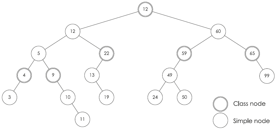
Furthermore in a PBST-n, a Simple node is the same as a Red node and a Class node is the same as a Black node in a RB Tree. This nomination helps to lift ambiguity and incomprehension of the main algorithm. This type of trees allows the representation of any order B-Trees.
Following the analogy between RB Trees and 2-3-4 Trees, there is the same analogy between B-nodes of order m and Classes of PBST-n where m = 2 n - 1. Therefore, we must preserve all properties of the trees. We define some basic operations simulating the rotations and color flips in RB Trees to insure the persistence of the B-Trees organization analogy.
4 Maintenance Algorithms
The organization of B-nodes is simulated in RB Trees by a set of Rotations and Color Flips where Rotations mimic the slide of values in a B-node and Color Flips the division and fusion of B-nodes. In PBST-n we simulate B-nodes of order in [2,2n - 1]. Furthermore, if we balance the tree on every node, this would give a perfectly balanced structure which would be just another algorithm form of RB Trees. Thus, to maintain such ideology and preserve the whole set of properties of the structure, the result of reflection gave an algorithm based rotation that insure a lower degree of balance and generalized form of RB Trees. This algorithm is based on three basic functions.
4.1 Restructuring
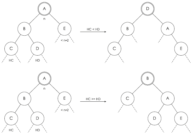
Restructuring is a set of rotations centered on the Class node that aims to slide the values of the Class when its height reaches the parameter n. It aims to distribute the values between the right and the left subtree of the class. Restructuring consists of one or two rotations depending on the situation of the class. These situations are defined by the height of one subtree is less than n - 2 and are illustrated in Fig 2 (other cases are found by symmetry):
— We use one rotation if the height of node C is greater than the height of node D. By applying a right rotation on node A, the height of the class is bound to be less than n.
— We use a double rotation when the height of node C is less than the height of node D. By applying a left rotation on node B followed by a right rotation on node A (a double rotation on node A), the height of the class becomes less than n.
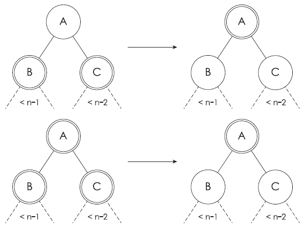
4.2 Partitioning
Partitioning splits the class into two subtrees. It mimics the division of a B-node. By changing the type of three nodes, the class is divided to two classes (Fig 3). Partitioning is invoked when both subtrees of the class are of height greater than or equal to n - 2 where Restructuring can't eliminate the obstruction of the third property.

4.3 Departitioning
Departitioning merges two classes into one class by changing the type of three nodes (Fig 4). It targets classes that have height less than n - 2 to merge with adjacent sister classes (By mimicking the fusion of two adjacent non-full B-nodes, such classes have less than half the values of a B-node).

5 Insertion in PBST
Insertion in PBST is as simple as any BST insertion followed by some rebalancing to insure the structure properties. Based on the imitation of B-nodes by classes, it is very easy to give an algorithm for insertion. We proceed like in any BST by finding the key's position on the tree, of course, this position must be a leaf on a leaf class. If the classes height exceeds the parameter n (the class overflows), we must rebalance the tree. As a result, we can summarize the insertion in two steps.
Step 1: It's a BST insertion in short. We search for the key's position which is a nil pointer, making it a leaf of Simple type on a leaf class. If the height of this last class becomes greater or equal to the parameter n (the class overflows), we undertake Step 2.
Step 2: We aim to eliminate the imbalance caused by the exceeded height. According to the overflowed class, we distinguish two cases.
Case 1: In the overflowed class, the Class node has a son with height less than n - 2. A Restructuring (Fig 2) is performed. If the height of the class remains equal to n, we partition it.
Case 2: In the overflowed Class, the Class node sons have height equal or greater than n - 2. A Partitioning (Fig 3) is performed.
This Partitioning results in giving the mother class a new key and increasing its height. This can lead to a series of Restructuring and/or Partitioning with the mother classes going up the tree creating a cascade phenomenon. As a consequence, we repeat Step 2 until no Partitioning is needed.
6 Delete in PBST
Delete in Red Black Trees appears so complicated and difficult because of all the different cases and maintenance operations. However, if we look at its B-Trees equivalent operations, it becomes so easy to understand. In the case of a generalized algorithm of RB Trees, the delete algorithm is easy to implement because of the ability to merge two classes simulating the merging operation of two B-nodes. Delete in PBST begins like in any BST, which is by searching for the key and eventually its substitute leaf and eliminating the leaf.
The elimination of the key could decrease the height of the class to less than n - 2 (the class underflows) which is analogue to having a leaf B-node with less than half the number of keys a B-node can hold.
This situation is considered as an imbalance on the tree and must be rectified. By merging the adjacent classes and redistributing the keys, we can eliminate such imbalance.
Thus, the delete algorithm is very simple and can be summarized in two Steps.
Step 1: we search for the key's position on the tree. If it is an internal node, we continue our search to find the immediately next value and permute the values. Then, we eliminate the node containing the key value. If the class from which we deleted the key underflows, we undertake Step 2.
Step 2: when a class underflows, we have to departition to keep the same load on the different parts of the tree. We distinguish three cases.
Case 1: the underflow class has a direct sister class with height smaller than n - 1 (Fig 5).
A departitioning is to be performed. We continue with the mother class and check if the class underflows.
Case 2: the underflow class has a direct sister with height equal to n - 1. (figure 6) A mere departitionnig results in a class with height equal to n. Therefore, we must restructure. We consider the sister classes and the parent as a class rooted at the parent (this can be done by simple changes of the types of the nodes). If the parent was simple, the new class is restructured. If the new class height is smaller than n, the delete process continues with the mother class as a node was removed. Otherwise, the obtained class is partitioned. If the parent was a class node, the new class is restructured and partitioned.

Case 3: the underflow class hasn't a direct sister class (see figure 7).

The property of partial balance guarantees the existence of a sister class. We have got to transform the tree to make it a direct sister. If the underflow class is to the right (resp. to the left) of the parent, the sister class is the first class found from the parent by going to the left (resp. to the Right), then to the most right class node (rep. to the most left). Transforming is equivalent to a simple rotation since only two pointers are modified. We modify the type of the parent and of the simple direct sister node.
7 PBST-2 as a Red Black Tree
PBST-n simulates the behavior of B-Trees in a binary tree form. Originally, Red Black Trees were created in order to define a binary representation of B-Trees of order 4. Thus, PBST-n should cover and are equivalent to Red Black Trees given the right parameter. This exclamation is easy to demonstrate as PBST-n are just a generalization of RB Trees. In fact, there is an equivalence between RB Trees and PBST-2. To simulate B-Trees of order 4, PBST classes must hold at most 3 keys limiting their heights to two nodes, one class and one simple. The same is observed on RB Trees, one Black and one Red. Furthermore, it is easy to show that the definition of PBST-2 is just another interpretation of Red Black Trees definition by using Class nodes as Black nodes and Simple nodes as Red nodes.
Proof: The definition of PBST-n when n=2 becomes just another formula to RB Trees. This can be demonstrated easily even if it is not obvious at first. PBST-2 is defined by:
(1) Each node is either a Simple or a Class node.
(2) Each direct path from Root to a leaf contains the same number of Class nodes.
(3) Each Class has a height of 0 or 1.
while RB Trees are defined by:
(a) Each node is either Black or Red.
(b) Each direct path from Root to leaf contains the same number of Black nodes.
(c) Each Red node must have Black children.
By taking into account that Black nodes are Class nodes and Red nodes are Simple nodes, the pairs of properties (1,a) and (2,b) are the same in the two definitions. The only property that isn't showing is the third property. Note that a class of height 0 or 1 is a class with a Class node and one level of Simple nodes at most.
Those Simple nodes have either Class nodes or the nil pointers as children. By taking the Black node hypothesis, those simple nodes have only Black nodes as children. Note also by taking Red nodes must have Black children, we find that in a RB Tree the Classes created by Black nodes have at most a height of 1. Thus, the two definitions are totally equivalent making the RB Tree as a particular case of PBST-n when n = 2 and verifying that PBST-n is a generalization form of RB Trees.
8 Analysis on Height
One major question with BST's is the performance threshold of the structure. As the performance is highly related to the balance of the trees, it is very important to define the degree of balance of the structure. As a binary based structure, the balance of BST's can be defined by the distribution and height of the structure. Actually, with a perfectly balanced tree, the height and distribution are just a logarithmic fraction to the number of elements of the set.
The height of the tree gives proportional information to the search time and consequently the update time. With lesser height, it requires fewer probes and as a result better performance.
8.1 Order of the Tree
Various BST's are compared to the B-Trees which are perfectly balanced trees on the node distribution level and the use of such BST's to represent B-Trees is one of the methods to define the optimization benefit from such structures. As B-Trees have a fixed relation to the number of restructuring operations, they give a decent scheme for comparison.
The generalization of Red Black Trees through PBST is based on the tolerance of finite successions of Red nodes analogically extending the binary representation of 2-3-4 Trees by Red Black Trees to higher order B-Trees where each B-node is represented by a Class (Black) node and its direct Simple (Red) descendants.
In fact, for various values of n , we can represent B-Trees of higher order by representing B-node of 2n - 1 by Black rooted subtrees of height n - 1. For example: PBST-2, trees can represent B-Trees with node up to 22 - 1 = 3 values; PBST-3, trees can represent B-Trees with nodes up to 23 - 1 = 7 values, …; and so on through the same analogy.
This representation suggests that the average height of PBST-n is n times the average height of the B-Tree it represent in the worst case which is a very good height considering the binary representation. As n is the logarithmic value to the width of the B-node, it is interesting to have such flexibility on the nodes with easy update operations compared to B-Trees.
8.2 Worst Height Case
It is difficult to define the balance of the tree however there is a practical way to know the degree of balance/imbalance of the structure through the establishment of precise intervals to the height of the tree. One way is to know the best and the worst possible height a structure can have for a set of elements (keys).
These two values give an interval to the height of the structure and create a margin to the distribution of its items. It is widely known that a perfectly balanced tree has a logarithmic height to the number of its items. Thus, we just need to have an overview on the worst height the structure can take.
Theorem. In a PBST-n, the worst case height is of n log (N + n) - n log n where N is the number of keys on the tree.
Proof: Let the height of the PBST-n be the maximal number of nodes
in any path from the root to a leaf. Then an PBST-n T
min(h) of height h with the minimum
number of nodes is of the form Fig. 8.
Notice that h = n.j where j
is the number of Class nodes in each path from Root-to-Leaf. The tree is bound
by two major conditions for every small tree rooted by a Class node. A small
tree of maximum height and minimum number of nodes is a vine of
n nodes (Class node included). And each node of the longest
path of the root small tree is linked to the root of a complete balanced subtree
of height
since
we obain
So the number of nodes of the tree N(T) is bound by:
which implies the in-equations:

The height of the PBST-n is at most n log(N + n) - n log n which is a little worse than RB Trees height 2 log (N + 2) - 2.
This could lead to a large difference in search time with large ordered sets. But considering the advantages of a binary representation, it is very interesting to have a low balanced structure. Furthermore, we gain some update time through the low rate restructuring.
8.3 Number of Restructuring
The tolerance of finite successions of Red nodes between Black nodes to define a generalization for Red Black Trees provokes some loss in balance. This, as shown in section 8.2, decreases the performance with the search time.
However, it is quite interesting for the update time as it accelerates the update time quite significantly. The number of Black nodes is decreased and consequently the number of maintenance operations that occur due to the cascade phenomena in insertion and delete.
Corollary. In a PBST-n, an update operation need at most log(N + n) - log n maintenance operations.
Proof: In the worst case scenario, the height of the tree is given as h = n log (N + n) - n log n, h = n.j where j is the number of Class nodes that may need balance maintenance due to the cascade phenomenon. Thus, the number of maintenance operations can, at most, reach j = log(N + n) - log n.
When comparing the number of Class nodes log(N + n) - log n to the number of Black nodes in Red Black Trees log (N + 2) - 1, it is clear that the number is decreased significantly and consequently the number of maintenance concerned nodes. This decrease in maintenance operations makes for faster updates as each operation is rather costly compared to the loss in search time.
Moreover in the overall view of performance, we find the generalized form competing with the Red Black Tree and considering various applications of such structure and environment, there is some situations where the generalized form is better.
9 Test Results
Performance of structures is one of the main debatable issues. To know the behavior of the structure doesn't suffice to tell the real threshold of its performance. This is, of course, due to the various distributions of keys it may be in contact with.
Thus, several researchers tend to define the performance through giving an estimate to the best and worst scenarios. In light of such ideology, we defined two scenarios where we believe this gives a general and relatively accurate interval of the different aspects of the generalized trees. The two scenarios are defined as follow:
— Scenario 1: we insert files of randomly generated/ordered keys of sizes N = {100, 200, 300, …, 900, 1000, 2000, 3000, …, 9000, 10000, 20000, 30000, …, 90000,100000,150000, 200000, 250000, …, 950000, 1000000}. Then we delete them.
— Scenario 2: we insert the same files as scenario 1. Then we use those files to check if each key is in the set, we delete it, else we re-insert it.
We took sets of 100 instances of experiments with each number N up to 90000 for parameter n = {2,3, ...,7} to define the structure behavior in distribution and 10 instances of experiments with 100000 ≤ N ≤ 1000000 to define the performance for bigger numbers. The results are quite interesting and define average values for search and update operations. It is expected that by losing in balance, we lose in performance.
However, the collected results show rather different observations. In fact when the keys are randomly generated, the difference in time performance is quite minimal. It is standard to define BST's performance through average and worst case height of the tree. But due to the former observation, we concluded that giving such estimate is necessary but not sufficient to define the whole story behind the performance and we tried to give/define the distribution of keys in each parameter tree.
In typical definitions of performance threshold, search time is the most important parameter as it constitutes the major part of the operations. With an almost null fail search fraction, the heights of the trees give a relatively accurate definition to this performance as it narrows the interval of expected results.
Furthermore, we observe that the search time (Fig. 9) is proportional to the height of the tree (Fig. 10). Both the search time and the height of the trees follow an exponential curve. In the case of randomly generated keys, the search time is almost the same between different parameters, the difference lies in the period of the change of the height that has a high relation to the parameter itself.
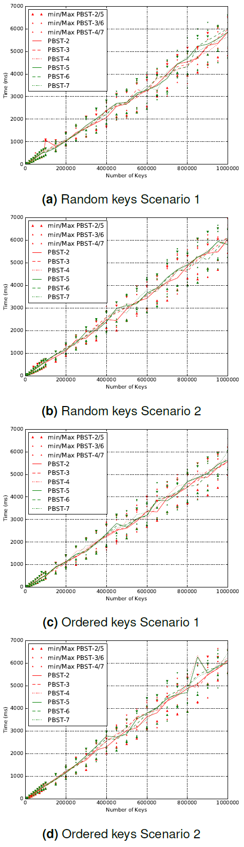

On the other hand, when the keys are ordered (as in the worst case), the height of the trees is increased by quite the amount provoking a loss in balance due to the change of the parameter, but the search time is almost the same. This result implies that the loss in balance doesn't affect the overall cost on the search time and that the average total search time gives a scheme to the expected average search cost. This cost is slightly the same for the various parameters.
Although, this remark might be inconceivable at first but it is explained by the height of the tree where it changes by 1 or 2 units at most between parameters insuring that the difference in search time is almost negligible and offering as a consequence the same level of performance for consultation.
As mentioned before, the search time and height performances are not sufficient to justify the use of different parameters. In fact, a highly imbalanced distribution can lead to lagging update operations with large restructuring phases. By design, PBST-n are less balanced the higher n parameter, allowing the possibility of having leaning trees to the right or left with unequal number of keys in the subtrees. The distribution of the tree can be described in about accurate manners through giving the root rank in Inorder traversal (Fig. 11), thus dividing the load on each subtree, or by giving the number of Simple (Red) nodes (Fig. 13) and the longest sequence of those type of nodes (Fig. 14). In the case of randomly generated keys, the root rank (Fig. 11) changes gradually in the same way within the different parameter trees. We see the same periodic evolution phenomenon in the case of ordered keys.


However, the fraction of the rank on the number of keys (Fig. 12) stays about the same through the different parameters with a considered amount of degradation in the case of ordered keys. In the general case by avoiding extreme distributions, the load of the tree is quite balanced between the left and right minimizing the effect of loss due to the increase in parameter.
On the other hand, we observe a gradual increase in the number of Simple (Red) nodes (Fig. 13) and the length of its maximum sequence (Fig. 14). Of course, this is explained by the properties of PBST-n, as n goes higher the length of its classes goes higher. This provoke a degree of imbalance but as a consequence the update operations require less maintenance operations and with random keys the loss due to imbalance is expected to drop showing little difference between the different parameters.
The acquired results show the same conclusion in both the insert (Fig. 16) and the delete (Fig. 18) operations. The update time (Fig. 15, 17) is improved by quite the amount on the operation scale giving a slight edge for the higher parameters. The gain in the number of restructuring and maintenance operations (Fig. 16, 18) is the rather significant observation.


In fact, the overall gain is really high to consider using higher parameters in environments where restructuring is more costly. The behavior of the trees is aligned to the development of their heights and the number of Class (Black) nodes. It is explained by the effects of the two phases of the update operations, the search is slightly affected by the imbalance but the restructuring is decreased drastically. We recognize a trade-off between the balance and the cost of maintenance suggesting the possibility of adapting the structure to different environments through the choice of parameter value.
10 Conclusion
We presented a new structure, called Partitioned Binary Search Trees (PBST), which aims to generalize the Red Black Trees by tolerating finite succession of Red nodes and presents a partitioned tree form by the use of class (Black) nodes. These trees offer a relaxed form for Red Black trees with high speed and low cost update operations. The relaxation is a result for the tolerated imbalance and cutting in the number of restructuring.
Although the height of the tree is slightly increased, the search time is of the same level. In fact, when the inserted keys sequence is not totally ordered, this effect is almost negligible. The height increase is explained by the increased number of Simple (Red) nodes giving a worst case scenario of n log (N + n) - n log n.
Moreover, the structure is interesting for its simple and easy to comprehend insert/delete operations. PBST-n, in its core, simulate higher ordered B-Trees. In fact, when n = 2 PBST-2 is equivalent to Red Black Trees. The experiments results show that in a random generated key environment the structure gives the same performance level of RB Trees with less needed restructuring suggesting a higher adaptability with environments of costly maintenance such as schedulers. Furthermore, the structure gives a quite balanced distribution if omitting the worst case scenario.
PBST-n allow the change of the parameter value that could be used to tweak the structure in order to save in update or regain balance by increasing/decreasing the value. It would be interesting if there was a way to have an auto-change of this value in relation to the trees balance and distribution.

