


 nueva página del texto (beta)
 Inglés (pdf)
 Artículo en XML
 Referencias del artículo
 Enviar artículo por email
 Citado por SciELO
  Similares en
SciELO
Similares en
SciELO 
 Permalink
1 Introduction
Maintaining fixed landmark visibility has been used in robotics to improve localization, navigation, object recognition, object manipulation, 3D reconstruction, quality inspection, etc. This task has been performed using motion planning, optimization, and visual-servoing techniques. Roboticists have recently focused on integrating these techniques [6,7]. In our approach the motion planning, with visual constraints, maintains landmark visibility and provides good landmark visual acuity.
1.1 Related Work
This approach is related to techniques that search the robot state space to develop collision-free and occlusion-free paths for eye-in-hand robots. In [6] the authors call these techniques path planning for visual-servoing. They also divide these techniques into four groups: (1) Image space path planning, (2) Optimization based planning, (3) Potential Field-based path planning, and (4) Global path planning. The approach is related to motion planning algorithms that impose physical and visual constraints to build a collision- and occlusion-free path.
Image space motion planning creates a path for the camera and then verifies path feasibility in robot configuration space. In [7], for example, the authors present an approach that partitioned the visual-servoing problem into one employing several sub-targets, to simplify the control task, when the main target is far from the camera.
The algorithm developed is based on the Rapidly Exploring Random Tree (RRT) approach. They first sample the image space and project visual features in the image. If the image space restrictions are satisfied then the tree is extended. The final camera trajectory is evaluated for configuration feasibility.
The principal disadvantage of image space motion planning is that suggested paths are not always feasible requiring re-planning until feasibility is obtained. To overcome this, some approaches have focused on planning in both image space and robot configuration space [11,1] simultaneously. In [11] the authors presented a motion planning algorithm for visual-servoing based on the RRT approach. The algorithm built an exploration tree, to encode robot configurations and visual features and obtain useful paths preventing target visual occlusion during the visual-servoing process. While, simultaneously, satisfying joints limitations and field of view restrictions. In [1] the authors present an algorithm to build an exploration tree searching in both image space and configuration spaces.
This algorithm plans the robot movements allowing no robot base positional alterations. Approaches like those presented in [11] and [1] are limited to generate feasible robot trajectories without attempting to find optimal trajectories. Additionally, these approaches were computationally expensive as they detect targets in an image. Their sampling-based planning algorithms must search a virtual environment, requiring virtual camera images to perform image space searches adding significant computational time to first build and then analyze and process these images. The approach presented in this work could be potentially combined with robot navigation methods like the one presented in [10] to maintain visibility of an object while the robot navigates in the environment.
Optimization techniques have been attempted to obtain optimal trajectories with respect to cost. In one example, optimization is done by 'cost minimization' considering the error between the length of a certain "feasible" path and the length of the straight-line path between any impose restrictions.
The optimization required two steps: first the translation vector and then the rotation matrix were optimized [2]. The principal disadvantage of this type of approach is that it is limited to simple (sub-four jointed) robot systems and environments with limited numbers of obstacles [6].
Our approach can be used in complex environments and with robots having many degrees of freedom. The algorithm has been tested in a six degree of freedom (DOF) manipulator, equipped with a camera having a limited field of view. This robot/camera machine was mounted in an environment populated with obstacles. Any of these obstacles could produce a robot collision or could occlude the landmark. The algorithm computes a collision- and occlusion-free path between two configurations. The landmark must remain visible during the execution of the entire robot path. Furthermore, the algorithm is able to optimize feasible robot paths by iteratively re-planning paths during the overall path planning process.
1.2 Main Contributions
The main contributions of this work are the following: We extend the RRT* to maintaining landmark visibility in an environment with obstacles, considering both motion and visibility constraints. We model this problem to either (1) respect some constraints, or (2) reach optimization, and compare the results. Visual features are inferred using a collision detector to determine whether an object is in the camera field-of-view and is occluded or not. We develop a technique that infers object visual features using a collision detector for any robot configuration. Camera roll angle (γi) was restricted to angles that limit changes in the landmark view orientation. Metrics for the RRT* algorithm include to minimize robot trajectory length, maximize the distance between the landmark features and the image boundary, and to minimize camera roll angle changes. Each of these algorithmic improvements have been implemented in both simulation and experiments with a 6 DOF ABB robot.
2 Problem Formulation
The robot is equipped with a camera with a limited field of view considering width, height and range. It is assumed that this camera is placed on the robot end-effector. It is assumed that the workspace is populated with obstacles and has a unique landmark (see Figure 1(a)).
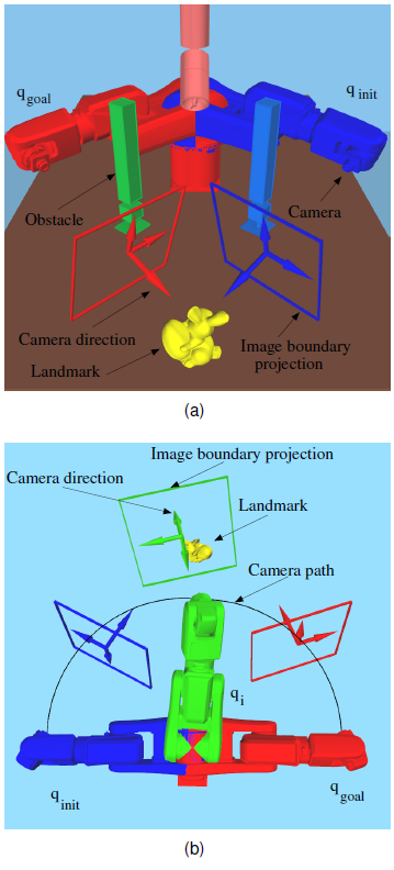
Fig. 1 (a)Robot and environment, (b)This figure shows the concept of maintaining visibility of a landmark. The initial robot configuration q init is represented with a blue robot (left) and the camera visibility at that configuration is represented with a blue frame (the image boundary projection). This frame is a slice of the camera field of view and the arrows represents the camera direction. The final robot configuration q goal is represented with a red robot (right). An intermediate robot configuration is presented in green (middle). The desired camera path is shown as the black arc and every robot configuration to achieve this path has the landmark in the camera field of view
2.1 Landmark Visibility Problem
The main problem addressed here is to maintain consistent landmark visibility while computing a collision- and occlusion-free path between an initial and final robot configuration (see Figure 1(b)). Requiring that the landmark remains in the camera field-of-view as the robot moves, remains un-occluded by objects, and motion occurs without physical robot-object or self-collisions, limits the number of paths that the robot could use as it moves in the environment.
Let C denote the robot configuration space for moving in a 3D world and V be a space that indicates whether the landmark is/isn't contained in the camera field-of-view v ∈ V as it moves. For each robot configuration q ∈ C there is a scalar that indicates whether the landmark is fully visible in the camera's view. Let Cobs be the obstacle region where the robot will collide with obstacles or itself, and let Cocl be a subset of C where the landmark is partially, or not, seen by the camera. Let Cfree be free configuration space where the robot is collision-free, and the landmark occlusion free (C \ (Cobs ∪ Cocl)). To build a planned solution, the algorithm searching for a path within Cfree space is required. The planning problem is to find this feasible path such that:
— A path is a continuous function, τ : [0,1] → C.
— A free path is a path in the free space τ → Cfree.
— A feasible path is a free path that starts at qinit and ends at qend ∈ Cgoal
Robot configurations on the feasible path are subject to physical and visual constraints: the robot is not in self- or obstacle-collision and the landmark is completely un-occluded in the camera field-of-view.
2.2 Landmark Visibility Constraint
A procedure was developed to assure no landmark occlusion that interfers landmark visibility. This procedure uses 3D models and a collision checker to infer whether the landmark is fully visible at a given robot configuration. Let O be a set of 3D models that represent all objects in the environment (including the robot itself at a given configuration - qi). In order to determine the landmark visibility the procedure builds a 3D frustum model, that represents the limits of the camera field-of-view, and a Ray-casting model, that represents rays from the camera center to the landmark in the environment ol ∈ O.
2.2.1 Detecting Objects inside the Camera Field of View
Let μi be a 3D model of a frustum that represents the camera field of view region. The frustum height is the perpendicular distance between the planes indicating near focal length and far focal length of the camera. The other four planar surfaces represent the camera's imaging limits. This model is attached to the robot end effector (see Figure 2). Thus, an object ol fully inside this frustum meets the visibility constraint if it is not occluded by another object oh. Let M be the space that indicates whether the landmark is or is not contained in the frustum as the robot moves. A scalar mi ∈ M is used to indicate this at a specific robot configuration qi. To map a configuration qi to a scalar mi a map is defined as M : C → M or in functional notation mi = M(qi). Here M is based on the collision checker that detects any "collisions" between a solid 3D model of μi and the landmark model ol.
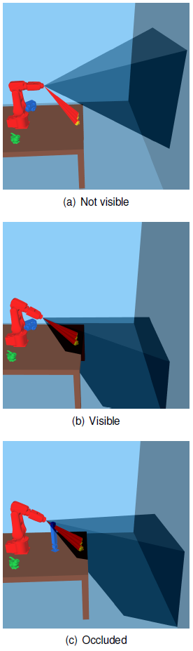
Fig. 2 Frustum model: camera frustum attached to the robot end effector. Ray-casting model: rays from the camera center to an object. (a) Landmark not visible by the camera: the Ray-casting model is not within the frustum model, (b) landmark visible by the camera: the Ray-casting model is within the frustum model, and (c) landmark occluded inside the camera field of view: the Ray-casting model collides with an object model
2.2.2 Detecting Landmark Occlusions
Let k1 be a 3D model that represents rays from the camera center to the landmark ol ∈ O (see Figure 2). If the ray-casting model k1 collides with an object model oh (for any h ≠ l) then the object oh is in between the camera center and the landmark, ol indicates landmark occlusion, regardless of whether ol is in the camera's field view or not.
Let K be the space that indicates whether the ray-casting model collided with objects models for each qi ∈ C. To map a configuration to a scalar ki that indicates whether the ray-casting model k1 collides with any object model oh (for h ≠ l) at that configuration, a map is defined as K: C → K. K uses a collision checker to detect occlusions.
This ray-casting model k1 is dynamically modified
while the robot moves, since the camera center pose changes with different robot
configurations. The ray-casting model k1 is
constructed using the landmark model ol and the
camera center p. The landmark model
ol uses a triangle language (STL file format)
for the 3D model representation, having j triangles. Each
triangle has three line segments:
2.2.3 Detecting Full Landmark Visibility
To infer landmark visibility at a given configuration qi the procedure searches in M and K. The landmark ol is fully visible at a given robot configuration qi if ol is completely inside the frustum and ol is not occluded.
Let V be a space that indicates whether the landmark ol ∈ O is fully visible as the robot moves. vi is a scalar that indicates landmark visibility, we define V: C → M × K → V in functional notation vi = V(M(qi), K(qi)). The map V determines whether the landmark ol is completely inside the frustum, and whether an object ol is visible by the camera. Each vi is a scalar that represents the landmark visibility. If the landmark ol ∈ O is not fully visible vi is zero.
In a feasible path τf, each qi ∈ τf has a vi equaling one, indicating that the landmark is fully (camera) visible.
2.3 Modeling Landmark Visibility
Sampling-Based Path planning in the Joint-Image Space (as in [5]) could be computationally expensive, since the workspace-image projection process would be done many times in the sampling and other primitives of the planning algorithm. In contrast we present a planning approach in the joint space with visual constraints built into the algorithm. These visual landmark feature (position/orientation) constraints, in the algorithm, are inferred using only workspace information without an image. How these visual constraints are included is explained below.
2.4 Landmark Visual Features Constraints
There are two main constraints to be respected. One wants to keep the landmark
'far' from the image boundaries and one wants that the orientation angle of the
image (camera roll angle), γi) to be close to a
specific value. Landmark distance to the image boundaries
To limit
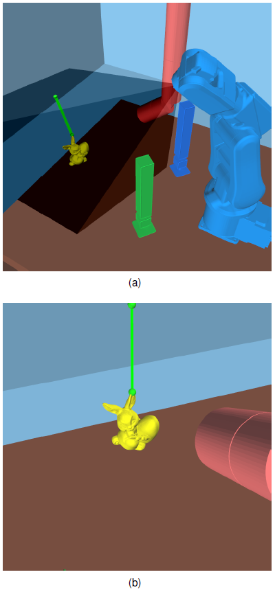
Fig. 3 (a) Distance between landmark model and the frustum model
di, (b) distance
between landmark features and image boudaries
To limit
3 Path Planning to Maintain Landmark Visibility
Sampling-based path planning algorithms can be extended to consider visual constraints by including them in the path planning algorithm. Here these visual constraints are used to extend the RRT* algorithm [3,4]. The problem of constraining the position and orientation of the landmark visual features in the image space can be modeled as either a problem of respecting some constraints or an optimization problem. Below, we present both formulations and compare the solution results.
In this path planning problem the RRT* algorithm searches in Cfree and uses information from V space, D space and Γ space in the algorithm primitives. In the original RRT* algorithm [3,4] an exploration tree of robot trajectories is incrementally built. The algorithm starts from a root that represents the initial robot state.
At each iteration, a random sample from the free-state space is chosen and the tree is expanded by adding a new node to the tree for this random sample. Besides, a process can change the structure of the tree to reduce the length of the trajectories from the root to the leaves by choosing paths with closer nodes (using this strategy the authors proved asymptotic convergence to global optimality [3]).
To deal with the planning problem, some primitives were modified to include visual constraints, they are described below. We consider that the configuration space is equal to the state space, that is X = C.
3.1 Primitive Procedures
In the list, unmodified primitives procedures, from [3,4], are summarized while modified primitives include more details.
— CollisionFree(xi) returns true (1) if the robot is not in collision with the environment (nor in auto-collision).
— LandmarkVisibility(xi) returns true (1) if the landmark is fully visible or false (0) otherwise. The visibility is computed using the map vi = V(xi) (see Section 2.2).
— SuitableFeatures(xi) returns true (1) if the landmark visual features fulfill the visual constraint (see Section 2.4) or false (0) otherwise. The function is based on the maps di = D(xi) and γi = R(xi) (see Section 2.2).
-
— StateValityCheker(xi) returns true if xi satisfy the physical and visual constraints, i.e., the following sentence is true:
For implementation purposes we established a state validity checker function to be used with the OMPL [12]. OMPL itself does not include code for this checking, it was intentional, since defining validity depends on the type of problems to be solved [12]. Here we define a state validity check considering collision checking between loaded CAD models, landmark visibility, and feature suitability.
-
— Sampling: SampleFreei is a map, from random variables, to points in the free state space Xfree. Here a random state xrand is determined to be in Xfree using the StateValidityCheker(xrand) function.
if xrand is not in (X)free a new random configuration is evaluated until xrand is in Xfree.
— Distance: Given two states: x, y ∈ X, the Distance function returns distance between the two states. The distance function is the L2 norm used for a State Space in OMPL.
— Nearest Neighbor: The function Nearest : (G, x) → v ∈ V returns the vertex in V that is "closest" to x in terms of the given distance function [3,4].
— Near Vertices: The function
— Steering: The function Steer : (x, y) → z returns a point z ∈ X such that z is "closer" to y than x is [3,4].
— Line(x1, x2) : [0, s] → X denote the straight-line path from x1 to x2[3,4].
-
— c(σ) is called the cost function, which assigns a strictly positive cost to all nontrivial collision-free paths [3,4]. Using this approach the cost function is:
where αc is a scaling factor, cc could be considered a clearance function imposing visibility constraints,
— Cost :
— Parent : V → V is a function that maps a vertex v ∈ V to the unique vertex u ∈ V such that (u, v) ∈ E. If v0 ∈ V is the root vertex of G, Parent(vo) = vo [3,4].
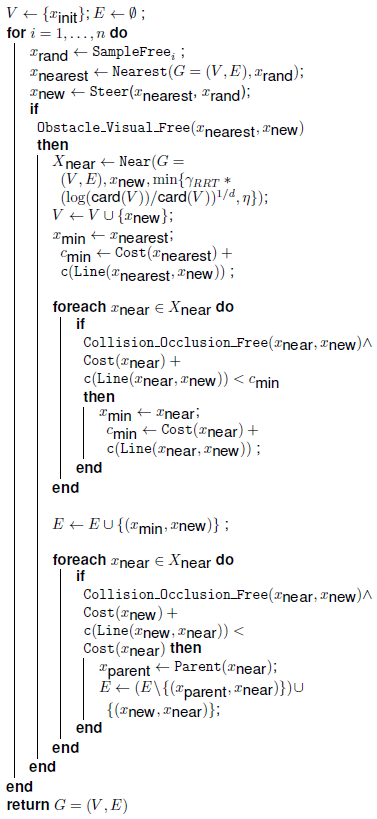
3.2 Algorithm 1: RRT* with a Landmark Visibility Constraints
We extended the algorithm RRT* from [3], to include visual constraints by modifying the SampleFree, ObstacleFree, CollisionFree, Cost and c primitives. The extended algorithm builds an exploration tree using the following steps ([3]):
3.2.1 Initialization (line 1, Algorithm 1)
The algorithm begins a search of the State Space by extending the tree starting at the root. The root depicts the initial robot state xinit and it is the first state of the path, e.i., τ(0) = xinit. We have assumed that the initial and final robot states are in Xfree.
3.2.2 Sampling (line 3, Algorithm 1)
The sampling process rejects every state x that is not in Xfree. In our approach we use the SampleFree function not only to check for collision free states but to check visual feature requirements directly associated to the states. The SampleFree function uses the StateValidityCheck function that was defined in OMPL by us.
3.2.3 Nearest Vertex (line 4, Algorithm 1)
The Nearest: (G = (V, E), x) function returns the vertex in V that is "closest" to x in terms a L2 norm (Distance) over the angles of two configurations. The distance function does not take into account the visibility features properties because the state space is the configuration space X = C. Since a configuration qi maps to vi, di and γi the state space X, here, is a subset of {C×V×D×Γ}.
3.2.4 Steering (line 5-6, Algorithm 1)
The function Steer returns a new state xnew, "closer" to xrand, from xnearest. The state xnew is an attempt to make a movement towards xrand. The state xnearesi and every node vi ∈ V fulfill the visual constraints, then xnew is also an attempt to maintain the visual constraints. To achieve this our Obstacle_Visual_Free function has extended the original ObstacleFree function in [3] and checks for both physical and visual constraints. If the landmark is fully visible and the landmark features are acceptable then an attempt to extend the tree towards xnew is made.
3.2.5 Extending the Tree (line 8-13, Algorithm 1)
Tests are performed to qualify the new vertex. A search for vertices near
xnew is done to connect it along a minimum-cost
path to G. The ratio r for the nearby vertices
is defined as follows:
The Collision_Occlusion_Free function is an extension of the original CollisionFree function in [3]. This function evaluates the validity of motions between two specified states. In our implementation, we perform a discrete motion validation.
The Collision_Occlusion_Free function uses the StateValidityChecker function to check intermediate states along the path between any two states. The disadvantage of this discrete motion validation is that the motion is discretized to some resolution and states are checked for validity only at that resolution. If the resolution is too large, there may be invalid states along the motion path that escape detection. If the resolution is too fine, many states must be checked, significantly reducing planner performance [12].
The state xmin is chosen between nearby vertices XNear having the minimum-cost path to xnew and the edge (xmin, xnew) is added to E.
3.2.6 Rewiring the Tree (line 14-17, Algorithm 1)
The algorithm modifies the tree structure looking for optimal trajectories between the root and the leaves as it rewires the branches of the tree. This part of the algorithm is also modified by including the Collision_Occlusion_Free function.
Using the c cost function, landmark features properties can be
optimized in terms of the visibility constraints imposed, that is
4 Results
We have tested our method using robot simulations and during experiments with a physical robot. OpenGL is used for visualization where all the objects in the environment are imported as 3D models using a triangle language. The PQP library is used to perform collision checking (and proximity query) and the Open Motion Planning Library (OMPL version 1.3.2) [12] is used to grow the exploration tree. Three different simulation experiments were performed to study some behavior differences in the RRT* algorithm with or without visual constraints. Physical experiments used a 6 DOF ABB IRB 120 industrial robot, which mounted a camera in its end effector, were also performed.
4.1 Simulations
The initial and final robot configurations are the same for the three simulation studies. The environment includes several colored objects (the robot arm, miscellaneous workspace objects and the target landmark). To enhance visualization, different colors are used for each robot configuration, blue represents the initial robot configuration, red represents the final robot configuration, and other colors represent intermediate robot configurations along the planned trajectory. The landmark can be any of the objects on the table, but for these simulations the rabbit (yellow) is the target landmark.
Once an acceptable path is found, a representation of the exploration tree and the planned path were displayed. The number of iterations n is not constant, and a time termination condition to the building process was employed. The following settings were used in the algorithm: a) k = 310 neighbors, b) r = 3.460682 for the near function, c) the range of allowed roll angle γi is [±1.2] radians, and d) the minimum allowed distance d is 0.125 decimeters.
The 3D models used in the algorithm are different from those used in the visualization. In order to reduce the computational time, the number of triangles was reduced, without losing their spacial properties, having the same (or more) space in the environment. The number of triangles for all models in O is 1422. Each simulation was run 10 times using an dual-core PC processor, equipped with 12 GB of RAM, while running Linux. Table 1 presents data obtained from the three simulations.
Table 1 *Average for successful simulation replay (data was rounded to fit with the column format). + No solution found within 300 seconds
| No. | Data simulation 1. Tree construction time: 60 seconds | ||||||||
| a) | b) | c) | d) | e) | f) | g) | h) | i) | |
| 1 | 7.5477 | 7.5477 | 22219 | 0.0902 | 0.3258 | 31454 | 15.61 | 16 | 8 |
| 2 | 7.1509 | 7.1509 | 22764 | 0.7290 | 0.5707 | 32124 | 15.56 | 74 | 42 |
| 3 | 7.3974 | 7.3974 | 23186 | 0.4697 | 0.2615 | 32724 | 13.23 | 35 | 24 |
| 4 | 7.3567 | 7.3567 | 22278 | 0.1482 | 0.5772 | 31453 | 14.37 | 20 | 14 |
| 5 | 7.2825 | 7.2825 | 22023 | 0.1729 | 0.2971 | 30973 | 19.07 | 61 | 44 |
| 6 | 7.5688 | 7.5688 | 22735 | 1.3700 | 0.4162 | 32063 | 13.56 | 13 | 10 |
| 7 | 7.6581 | 7.6581 | 22477 | 0.1594 | 0.5461 | 31559 | 9.8 | 212 | 127 |
| 8 | 7.4410 | 7.4410 | 22704 | 0.2378 | 0.2431 | 31989 | 16.21 | 39 | 22 |
| 9 | 7.3737 | 7.3737 | 22617 | 0.2542 | 0.4674 | 32029 | 23.11 | 46 | 26 |
| 10 | 7.4715 | 7.4715 | 22616 | 0.1726 | 0.2193 | 31772 | 18.19 | 43 | 22 |
| Avg.* | 7.4248 | 7.4248 | 22562 | 0.3804 | 0.3924 | 31814 | 15.87 | 56 | 34 |
| No. | Data simulation 2. Tree construction time: 300 seconds | ||||||||
| a) | b) | c) | d) | e) | f) | g) | h) | i) | |
| 1 | 10.6524 | 10.6524 | 732 | 0.7674 | 0.6635 | 182692 | 17.24 | 35581 | 62 |
| 2 | 11.5656 | 11.5656 | 667 | 1.2543 | 0.8583 | 192597 | 16.39 | 62806 | 89 |
| 3 | 10.7644 | 10.7644 | 663 | 0.7720 | 0.4064 | 184880 | 12.7 | 90750 | 219 |
| 4 | 10.6349 | 10.6349 | 546 | 1.0164 | 0.6379 | 166472 | 11.09 | 114531 | 319 |
| 5+ | -- | -- | 585 | -- | -- | 173070 | -- | -- | -- |
| 6+ | -- | -- | 483 | -- | -- | 189391 | -- | -- | -- |
| 7 | 11.0985 | 11.0985 | 664 | 0.9479 | 1.2133 | 195412 | 12.77 | 158143 | 475 |
| 8 | 11.0551 | 11.0551 | 691 | 0.8394 | 0.9365 | 221721 | 13.18 | 131034 | 298 |
| 9 | 10.3645 | 10.3645 | 654 | 0.8748 | 0.4753 | 207046 | 10.65 | 140441 | 350 |
| 10 | 10.5552 | 10.5552 | 646 | 0.7832 | 0.5133 | 198166 | 14.25 | 87829 | 151 |
| Avg. * | 10.8363 | 10.8363 | 658 | 0.9069 | 0.7131 | 193623 | 13.5338 | 102639 | 245 |
| No. | Data simulation 3. Tree construction time: 300 seconds | ||||||||
| a) | b) | c) | d) | e) | f) | g) | h) | i) | |
| 1 | 13.3081 | 136.6444 | 177 | 1.5365 | 0.2233 | 464135 | 175.43 | 273083 | 50 |
| 2 | 12.1779 | 97.7025 | 207 | 1.6387 | 0.0590 | 382945 | 176.62 | 103776 | 25 |
| 3 | 12.5840 | 121.5798 | 118 | 1.6573 | 0.1802 | 377586 | 190.55 | 258968 | 60 |
| 4 | 11.1268 | 113.9140 | 193 | 1.3177 | 0.1373 | 386441 | 179.45 | 142352 | 33 |
| 5 | 13.1672 | 119.3063 | 208 | 1.6610 | 0.1579 | 808397 | 216.11 | 568303 | 74 |
| 6 | 12.1210 | 107.3488 | 213 | 1.6865 | 0.1153 | 421746 | 226.45 | 82143 | 11 |
| 7 | 11.2181 | 107.9794 | 219 | 1.3503 | 0.0864 | 577084 | 171.97 | 198520 | 25 |
| 8 | 13.6679 | 113.0791 | 227 | 1.7191 | 0.0800 | 454258 | 190.07 | 113753 | 16 |
| 9 | 10.8290 | 95.9823 | 185 | 1.4427 | 0.0747 | 447962 | 102.27 | 297352 | 82 |
| 10 | 11.2491 | 107.5465 | 219 | 1.4734 | 0.1512 | 426150 | 176.65 | 126305 | 32 |
| Avg. * | 12.1449 | 112.1083 | 197 | 1.5483 | 0.1265 | 474670 | 180.56 | 216456 | 41 |
Legend: a) path length, b) path cost, c) number of vertices in the graph, d) average of the roll angle, e) average d distance (decimeters), f) number of iterations, g) initial solution path length, h) initial solution number of iterations, i) initial solution number of vertices in the graph.
4.1.1 Simulation 1: RRT* without Visual Constraints
The robot's task was to move the camera from the table's right to left side while avoiding collisions. This simulation was performed 10 times with a 60 seconds time limit. All ten simulation replays reached a solution within the time, see Table 1. Figure 4 shows the results of one simulation execution using the RRT* algorithm without visual restrictions. Figure 4(a) displays a representation of the exploration tree were every node in the graph (in white) is the camera position at any state in the tree. Figure 4(b) presents the planned path, each node in the path represents the robot camera and a segment line (in black) indicated the chosen camera positional transition between states.

In this simulation, at times, the landmark is fully or partially occluded by an obstacle so is not completely visible by the camera. Figure 4(c) shows a robot state where the landmark is occluded while Figure 4(e) shows a robot state where the landmark is not completely inside the cameras field-of-view. This was anticipated since during this simulation the algorithm searches only for a path without obstacle collisions regardless of landmark visual quality.
4.1.2 Simulation 2: RRT* with Visual Constraints and Only Path Length Pptimization
In the initial and final robot configurations, the physical and visual constraints are satisfied. In this simulation the robot's task was to avoid collision with the obstacles and to maintain the complete landmark camera visibility while the robot traverses the table's right side to its left side. The environment includes a 'lamp' that could easily occlude the landmark from many robot configurations (see Figure 5). This obstacle limits the occlusion-free robot motions since it is in between the landmark and the robot. Figure 5(a) presents the exploration tree.

Fig. 5 Simulation 2: (a) Exploration tree built using Algorithm 1, (b) the solution path to keep the landmark visible (only the camera path is displayed but the solution is a set of robot states where the landmark is always visible), (c) - (f) a robot configuration and its camera image in the solution path.
In this experiment there are fewer nodes than in the previous experiment (See Figure 4(a) of the Simulation 1) since fewer configurations will meet the imposed visual constraints. To maintain landmark visibility, the algorithm found a feasible path, but the camera had to be rerouted below the bottom edges of the lamp to avoid collision and landmark occlusion (see Figure 5(b)). As required, the landmark was always completely visible over the planned path. Additionally, landmark features are never too close to the image boundary and the landmark orientation is within the acceptable range. Figure 5(d) shows a camera image, with the landmark close to the image boundary, as the robot moved over the path.
Note here, landmark features could be close to the image boundary since the visual constraints only guaranteed that a minimal distance from the boundary of the camera field-of-view frustum is assured. Figure 5(f) shows a camera image indicating the maximum roll angle found over the planned path, which is within a range of valid angles. For this simulation, 10 replays were performed with a time limit of 300 seconds. A complete trajectory solution was found in 8 of 10 executions. Table 1 includes data obtained from the 10 simulation experiments.
4.1.3 Simulation 3: RRT* including Visual cost Optimization, the Landmark is as far as Possible from the Image Boundary and the Camera Roll Angle Close to Zero
In this simulation, a landmark visualization optimization process was added. The optimization was designed to assure that the landmark features remained as far as possible from the image boundary and the landmark γi change was minimized. Thus, Here robot's task is avoid collision with the obstacles, avoid occlusion and keep the landmark (nearly) centered and 'upright' in the camera field-of-view while the robot moves from table's right to left side.
While Simulation 1 and 2 are included for comparison, this third simulation was wholly based on the newly developed optimal path planning approach we suggest. Figure 6(a) presents the exploration tree. Since Cfree is the same for the Simulation 2 and 3, the exploration tree can be seen to be similar to Simulation 2.
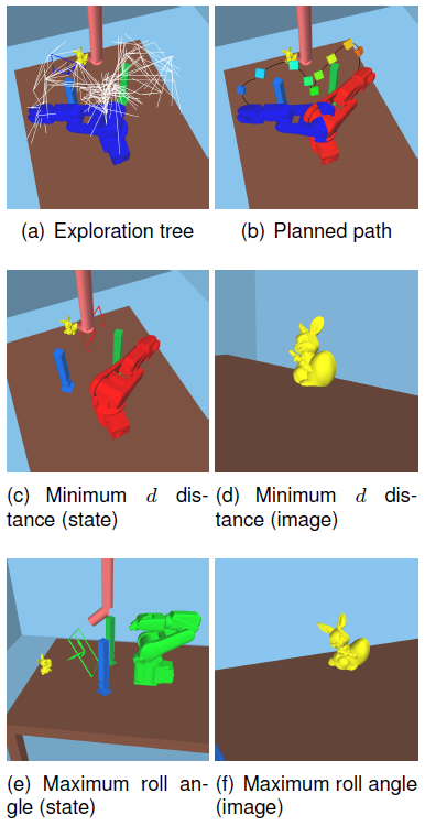
Fig. 6 Simulation 3: (a) Exploration tree built using Algorithm 1, (b) the solution path to keep the landmark visible and away from the image boundaries), (c) - (d) the initial robot configuration and its camera image in the solution path
Figure 6(b) presents the planned path. However, since the optimization process metrics had changed, the landmark features are closer to the center of the field-of-view and orientation is closer to the desired γi (zero) when compared to Simulation 2. Figure 6(d) shows a close up image of the landmark as it would be seen across the planned path. The landmark is nearly centered (as required for optimality) in the image.
Figure 6(f) shows the image at the maximum γi over the planned path, again, as required by the optimality constraints, it is nearly zero radians. For this simulation, 10 executions were performed with a time limit of 300 seconds. A complete trajectory solution was found in 10 of 10 executions. Table 1 includes data obtained from the 10 simulation experiments. We include a video of simulations 2 and 3 in the multimedia materials of this paper.
A video showing simulations 2 and 3 is also in the following link:
Link to the video: https://figshare.com/s/44616081306de618023d
4.1.4 Analysis
In this section, an analysis of the simulation experiments is presented. We call the simulation runs an experimental set, thus 10 trajectories, to connect the initial configuration with the goal configuration, were developed, note that some runs may fail to reach the goal, so all run results can be averaged. In simulation 1, only controlled by collision avoidance, in simulation 2 both collision avoidance and visual constraints are maintained, with path length optimization. In simulation 3, the visual features cost is added to the optimization process.
In our simulation notation, the distance d is the distance from the landmark to the field-of-view boundary. We consider an iteration one attempt to connect a new configuration to the tree. To obtain planned paths, we let the RRT* algorithm run for some prescribed time. In the case of Simulation experiment 1 we let the algorithm run for 1 minute, in the cases in which we satisfied visual constraints or optimize visual acuity (simulations 2 and 3), we let the algorithm run for 5 minutes, since many fewer potential configurations could satisfy the requirements.
We call first solution to the first path obtained by the algorithm that connects the initial and final configuration obtained within the time interval. Note that since the RRT* algorithm asymptotically optimizes the cost, the fist solution shall typically have a less good cost compared with the one obtained at the end of the time interval.
Table 1 (A. Simulation 1, B. Simulation 2, C. Simulation 3) contain data obtained from the simulations. Columns a) and b) shows the overall path length and path cost obtained after the RRT* was run over the entire time interval (60 seconds or 300 seconds for simulations 1, or 2 and 3, respectively). Column c) shows the number of vertices in the tree after the respective construction times, the number of vertices is smaller in simulations 2 and 3 since there are significantly fewer states that meet the visual constraints. Columns d) and e) shows the average of the d distance and the γi angle computed over the path configurations. Distances are larger and γi are smaller in simulation 3 because the optimization procedure maximizes the d distances (remembering this is the distance away from field-of-view boundary) and minimizes γi.
Columns g) to i) shows data for the first solution found at each simulation replay. Column g) shows first path cost, as expected it is greater than the path cost obtained at the end of the prescribed time reported in column b). Column i) shows the number of vertices of the tree, it is smaller than the number in column c). This is because the first solution is further optimized by the RRT* in the remaining time. Column h) shows the number of iterations; the number of iterations to find a first solution path increases in simulations 2 and 3 due to the visual constraints. However, the first and final solutions are found within the 300 seconds.
For each solution path, the d distance and γi were each used to create histograms for the simulations (see Figure 7). We compared the simulations histograms and noticed important behavior differences between them. Figure 7(a), the histogram of d distance for simulation 1, displays many zeros since every time the landmark is not completely visible the d distance is set to zero. The distance trend, as expected, closes on zero appears since no attempt to force full visibility was enforced. Figure 7(b), the d distance histogram of simulation 2 shows a tendency for keeping d above zero value, meaning that the landmark is always inside the frustum the same but higher d distances are observed in Figure 7(c) for simulation 3 since the optimization employed drove solutions with the landmark near the center of the frustum slice boundaries.
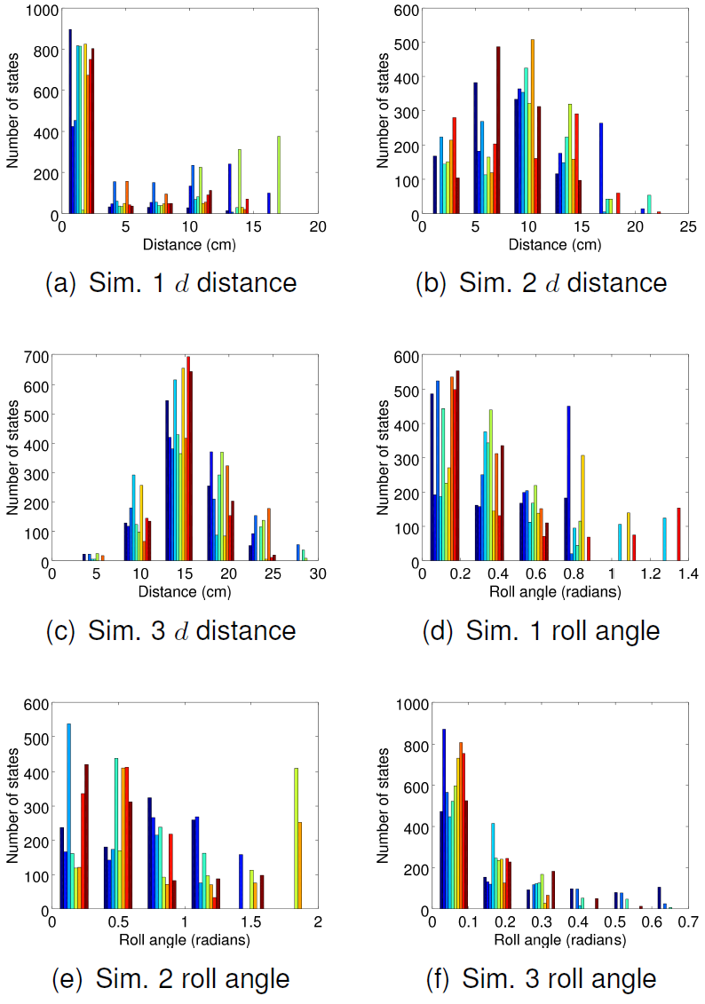
Figures 7(d) and (e) shows the histograms for γi during simulation 1 and 2, notice the similarities. The histogram of γi, in Figure 7(f) for simulation 3, clearly shows that γi is forced to be nearly zero. Thus, including a visibility (penalty) cost in the optimization procedure leads to a significant reduction in γi.
4.2 Real Environment
Our approach was tested is a real environment using an ABB IRB120 robot. The following settings were used in the algorithm: a) k = 310 neighbors, b) r = 3.460682 for the near function, c) the range of allowed roll angle γi is [±0.3] radians, and d) the minimum allowed distance d is 0.5 decimeters. The sum of triangles for all models in O was 408. Figure 8(a) shows the simulated environment. We ran the planner 10 times and chose a solution path, this path is shown in Figure 8(a).
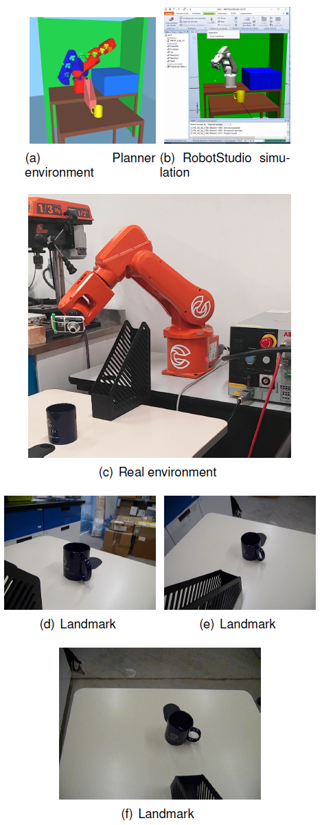
Table 2 contains data obtained from the planner. In this table, the number of iterations in 300 seconds is greater than in Simulation 3; this is due to the smaller number of triangles used in this experiment. Figure 8(b) shows the environment simulated in ABB's RobotStudio software; the planned path was successfully implemented and no collision was detected. Figure 8(c) shows our laboratory, the computed path was executed in this lab using the ABB robot. Figures 8(d)-(f) show eye-in-hand images captured during robot execution.
Table 2 *Average for successful planner replay (data was rounded to fit with the column format)
| No. | Data experiment. Tree construction time: 300 seconds | ||||||||
| a) | b) | c) | d) | e) | f) | g) | h) | i) | |
| 1 | 5.4281 | 43.7794 | 469 | 0.0614 | 1.6668 | 6430283 | 71.37 | 608875 | 11 |
| 2 | 5.6538 | 42.3186 | 479 | 0.0516 | 1.8007 | 5857054 | 62.78 | 523254 | 18 |
| 3 | 5.6362 | 44.5623 | 474 | 0.0534 | 1.7392 | 6342627 | 76.3 | 185366 | 6 |
| 4 | 6.4968 | 43.7135 | 472 | 0.0664 | 2.1811 | 4964429 | 107.69 | 49948 | 4 |
| 5 | 6.1990 | 44.9021 | 526 | 0.0466 | 1.8027 | 6258154 | 87.74 | 234877 | 3 |
| 6 | 5.9428 | 47.1370 | 479 | 0.0617 | 1.7480 | 5445362 | 70.7 | 515437 | 5 |
| 7 | 5.8550 | 44.6246 | 481 | 0.0506 | 1.7358 | 4908820 | 73.4 | 203507 | 5 |
| 8 | 5.9621 | 42.9004 | 567 | 0.0659 | 2.0306 | 7509052 | 63.35 | 166999 | 4 |
| 9 | 5.8253 | 44.0943 | 508 | 0.0652 | 1.7688 | 6578829 | 54.07 | 245903 | 5 |
| 10 | 5.3815 | 43.8238 | 493 | 0.0320 | 1.6382 | 5927889 | 67.89 | 259264 | 7 |
| Avg. * | 5.838 | 44.1856 | 495 | 0.0555 | 1.8112 | 6022250 | 73.53 | 299343 | 7 |
Legend: Real environment. Data are obtained from the planner replays: a) path length, b) path cost, c) number of vertices in the graph, d) average of the roll angle, e) average d distance (decimeters), f) number of iterations, g) initial solution path length, h) initial solution number of iterations, i) initial solution number of vertices in the graph.
The paper multimedia material presents a video sequence captured by the camera mounted in the robot end effector, while the robot executed the planned path. These experiments demonstrate that our approach can be successfully implemented to obtain an optimal path using a real robot, provided that 3D models of the obstacles are available. A video showing the experiments in the real robot is also in the following link:
Link to the video: https://figshare.com/s/44616081306de618023d
5 Conclusions
We propose and implemented a variant of the RRT* algorithm to include landmark feature constraints (see Section 4.1.2). We further developed a RRT* variant that further constrained landmark features to be inside the camera field of view but closer to the image center. This was accomplished by including a distance metric optimization routine (see Section 4.1.3).
Finally, we built a roll angle γi optimizer to limit its range forcing the visual features orientation to remain as undisturbed as possible during path execution. The presence of obstacles increases the computational difficulty for robot moves in cluttered environments but we were able to solve the problem in reasonable time. We successful built planned trajectories that avoided obstacle- and self-collisions, optimized landmark observation (non-occluded and field-of-view centric), finding desired trajectories in reasonable processing time (in the order of some minutes using a standard desktop PC).
We presented solutions for environments represented with 1422 triangles (used in the algorithm for all models in O) determined in under 300 seconds. We also present experiments that proved that our approach can be successfully implemented in a real robot, provided that the 3D environment models are known.
Only a few approaches had focused on motion planning for an eye-in-hand robot using visual constraints. Most of these approaches used visual features from an image to infer occlusion or to impose visual restrictions. In our approach, a collision checker is used to infer object visibility using workspace information. This is crucial for any efficient search algorithm in X. In this work we proposed to use a collision checker to infer the objects visibility, a proximity query package to compute landmark distance from a field-of-view frustum boundary, and homogeneous transformations to computes the roll angle γi.
Like most motion planning approaches, the algorithm depends on the availability of 3D environmental models and it can be used in real robot applications when a reliable representation of the expected environment had been prepared.
During future studies, we propose to develop an algorithm to maintain visibility of several visual landmarks for operation of mobile-based manipulator robots.

