


 text new page (beta)
 English (pdf)
 Article in xml format
 Article references
 Send this article by e-mail
 Cited by SciELO
  Similars in
SciELO
Similars in
SciELO 
 Permalink
1 Introduction
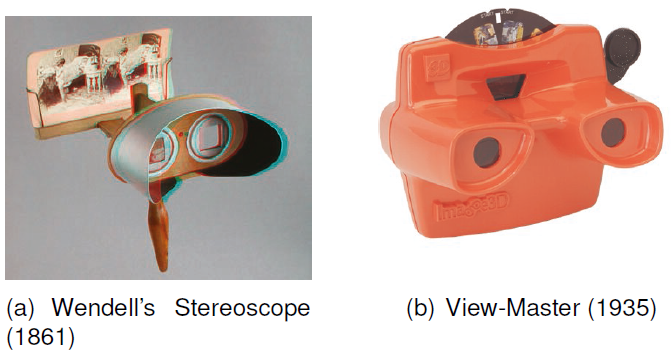
Stereoscopic coding and visualization systems are now an interesting field of research, but since the nineteenth century, several researchers presented some devices that displayed stereoscopic images. The Wendell's Stereoscope (Fig. 1(a), built in 1861) or View-Master (Fig. 1(b), commercially since 1935) are a good example of these devices. These devices captured two offset pictures (stereo-pair) separately showing left and right views to the appropriate eye of the observer. Then, when both views are combined into the brain, by means of stereopsis of binocular vision, they give the illusion of depth.
In general, these kind of stereoscopic past systems had 3 phases:
Nowadays, these stages have not changed, since they are just digitalized. Today, we capture stereoscopic images with digital cameras instead of plate cameras, we use polarized glasses instead of using anaglyph ones and the screen is no longer a piece of cardboard or reel, now it is a 3D television or 3D IMAX Screen.
Figure 2(c) shows the anaglyph image of My heart is a jungle (Fig. 2(a)), if this image is seen with anaglyph glasses, we could perceive it in different slices which depend on the apparent distance. This effect is similar like watching a version of its diorama, but digitalized(Figure 2(b)).

Maybe in future, stereoscopic scenarios with volumetric appearance and high quality will be part of everyday life, but now three-dimensional content is not simply a digital diorama, therefore the current challenge for researchers is to incorporate features based on the Human Visual System (HVS) for improving realism and immersiveness.
A general scheme of stereoscopic image quality assessing is depicted by Figure 3 (green block) and it is constituted by the following components:
Input: Stereoscopic Image, i.e. Left and Right views,
Process: Coding of Stereoscopic Algorithm ,
Output: Stereoscopic Representation of 3D Image, and
Feedback: Stereoscopic Image Quality Assessment (SIQA).

According to general systems theory, Feedback makes sure the efficiency of the Process [4]. So, the main objective of the SIQA is to quality assessment in the Left and Right views, then we can establish the degradation of the original stereo-pair. Coding of Stereoscopic Algorithm is to obtain the less possible degradation or fluctuations in the original source. Which is why, any kind stereoscopic image algorithm used in 3D projections, supports its evaluations employing a SIQA. So, we can recent evolution of stereoscopic algorithms is highly correlated with the evolution of the way to assess its visual quality. In this way, these methods of assessing stereoscopic quality have grown not only in number but also in importance.
The SIQA methods are based on the fact of evaluating two, or more, views of the same scene and the most of them employ either a 2D Image Quality Assessments (2DIQA) or slight adaptation of some HVS characteristics.
In this sense, it is reasonable to define SIQA as a variation of a 2DIQA, since in psychophysical experiments, the human observers subjectively assess the image quality [29,13,41] evaluating quality from a digital diorama, Figures 1(a) or 2(b), with lack of volumetric information of the scene.
SIQA algorithms can contribute to predict not only an objective response in general correlated with HVS but also the visual discomfort of an observer. In the early fifties, 3D Cinema was synonym of sickness and dizziness, sixty years later is related to blockbusters like Avatar [6].
Therefore, this paper is intended not only for SIQA researchers but also for researchers who study the visual discomfort or classical 2DIQA algorithms, since we classify and describe the most important features of SIQA algorithms and their combination with 2DIQA, resulting 280 metrics. Then, the main objective of this paper is to describe, in a general way, several SIQA algorithms in addition to compare them with the recent psychophysical experiments in the field. Which is why, we divided this work in four parts:
2 Stereoscopic Image Data Bases
In SIQA field exists few image databases. Thus, in this section we highlight some features of the most used image databases in addition to mention some features of their psychophysical experiments, which contain standardized procedures from [20].
The stereoscopic images quality data obtained by these kind of experiments are based on the opinion score of an observer of individual quality judgments, which builds the database (Figure 3, blue block). Each attempt, the images are classified on a variable scale from excellent to bad. Then, making use of most common statistical metrics such as mean, standard deviation or variance, data are analyzed, giving as a result the Mean Opinion Scores (MOS). Different statistical procedures can be applied in the MOS of every stereoscopic image database psychophysical experiments, so we recommend to consult the citation for knowing them. Furthermore, MOS concentrates experimental results, which allow the description or comparison of any kind of stereoscopic assessment metric.
On the one hand we want to present three of the most used stereoscopic image databases:
— LIVE 3D: Laboratory for Image and Video Engineering of the University of Texas at Austin (USA) Stereoscopic image database the proposed by Moorthy et al. [29], available at http://live.ece.utexas.edu. Figure 4 shows the 20 Reference images used in this subjective study, shown only the left-views.
— MMSPG: Stereoscopic image database of the Multimedia Signal Processing Group of the Ecole Polytechnique Federale de Lausanne (Switzerland) proposed by Goldmann et al. [13], Figure 5 shows four samples of reference images (only Left-views) used in this subjective study and it is available at: http://mmspg.epfl.ch/.
— FISE: Stereoscopic image database of the Faculty of Information Science and Engineering of the Ningbo University (China) proposed by Wang et al.[41]. Figure 6 shows four samples of reference images (only Left-views) used in this subjective study. It is important to mention that [41] collected the imagery from the work made by [34], and they took just 2 of the 7 views that this image database originally had in order to have a stereo-pair [17] and it is available at: http://vision.middlebury. edu/stereo/.

Fig. 4 Left-images of the 20 source or reference views used in the subjective assessment (LIVE-3D) of Moorthy et al. [29]


It is important to mention these three databases are not the only projects realized in the 3D/stereoscopic field. For example, [32] and [18] proposed another databases intended for improving the stereoscopic image quality. Both MMSPG and FISE image databases are not consistent with the size of reference and distorted images, since in some cases the size is different. So resizing images could change the precision of the subjective results. Thereby, this paper compares the psychophysical experiments of the LIVE 3D image database against a collected set of SIQA.
We want to mention their main features. Table 1 depicts the main characteristics of LIVE 3D, MMSPG and FISE image databases, where column Features refers to:
— Reference Images: Number of original or reference stereo-pairs.
— Distorted Images: Number of distorted stereo pairs.
— Format Images: Storage format of original and distorted stereo-pairs.
— Studio Images: Were the images captured in controlled conditions? Yes=Studio Images and No=Outdoor Images.
— Resolution: Size both for Reference and Distorted Images.
— Views: Views of the same scene.
— Distortions: Number of distortions, in the case of FISE are JPEG2000(JP2K), JPEG, Additive White Gaussian (WN) and Gaussian Blur (Blur). LIVE 3D use all these four noises in addition to Fast-Fading (FF).
— Observers: The subject pool considered in the study.
— Camera: Brand and model of the used camera.
— Capture Process: Simultaneous and Not-Simultaneous mean respectively that pictures were captured at the same time or not.
— Stereoscopic Display: Brand and model of the used stereoscopic display.
Table 1 Main features of LIVE 3D, MMSPG and FISE stereoscopic image databases
| 3D Image Database | LIVE 3D | MMSPG | FISE | |
|---|---|---|---|---|
| Features | ||||
| Reference Images | 20 | 10 | 10 | |
| Distorted Images | 365 | 100 | 20 | |
| Image Format | BMP | PNG | PNG | |
| Studio Images | no | no | yes | |
| Resolution | 640 × 360 | 1920 × 1080 | 1390 × 1110 | |
| Views | 2 | 10 | 2 | |
| Distortions | 5 | Not specified | 4 | |
| Observers | 32 | 20 | 20 | |
| Camera | 1 × Nikon D700 | 2 × Canon HG20 | 1 × Canon G1 | |
| Capture Process | Not-Simultaneous | Simultaneous | Not-Simultaneous | |
| Stereoscopic Display | Viewsonic IZ3D | Hyundai S465D | Not specified | |
It is important to mention that this work is adequate to judge exclusively stereoscopic images containing so-called 2D artifacts, since all the artifacts of LIVE 3D, MMSPG and FISE image databases are 2D artifacts added separately and symmetrically to stereoscopic scene, i.e. the left and right images.
3 Classification of 3D/Stereoscopic Image Quality Assessments
Before describing a certain SIQA algorithm, we propose a classification. Note that there are many possible classifications and we just expose three of them.
Table 2 shows the 27 metrics from 17 authors described in this paper. It is important to highlight that we maintain the name of the image quality assessment that author gives it, in addition some of these author propose more than one metric. Independently of the author, a certain metric is referred by its name taking in to account in its corresponding row.
Table 2 Stereoscopic Image Quality Assessments
| Algorithm | Metric |
|---|---|
| Akhter et al.[1] | AkMOSp |
| Benoit et al.[3] | d1 |
| d2 | |
| d3 | |
| Ddl1 | |
| Bosc et al.[5] | Qs |
| Campisi et al.[7] | Av |
| Va | |
| Chen et al.[9] | Cm |
| Gorley et al.[14] | SBLC |
| Gu et al.[15] | ODDM4 |
| Hewage et al.[16] | PSNRedge |
| Jin et al.[21] | MSEms |
| MSEdp | |
| Joveluro et al.[22] | PQM3D |
| Mao et al.[24] | Qmao |
| Shao et al.[35] | Qshao |
| Shen et al.[38] | HDPSNR |
| Solh et al.[39] | 3VQM |
| Yang et al.[48] | IQA |
| SSA | |
| You et al.[49] | YouDMOSp |
| OQ | |
| DQmap1 | |
| DQmap2 | |
| DQmap3 | |
| Zhu et al.[53] | ei |
Thus, in this section all metrics in Table 2 are classified, then in section 4 they are described and in section 5 they are tested. Also, SIQA-SET will be call henceforth to the set of these 27 metrics.
Historically, several authors such as [45] describe the taxonomy of 2DIQA algorithms as follows:
— Full-Reference (FR): FR metrics gauge the quality of a presumably recovered or distorted image or view giving as a result a complete knowledge of the original or reference source.
— Reduced-Reference (RR): RR metrics predict the quality of a presumably recovered or distorted image or view giving as a result an incomplete knowledge of the original or reference source.
— No-Reference (NR): NR metrics assess the quality of a presumably recovered or distorted image or view without any knowledge of the original or reference source.
This classification cannot exactly be applied in the same from in the SIQA field, since it is impossible to obtain either original or distorted stereoscopic images, simply because they are perceived by a human observer. In this way, we are not able to obtain the cyclopean image that is formed in the brain of the human beeing and we just can obtain information from left or right views of the so-called stereoscopic scene in order to predict other features, including the depth map.
Thus, our first classification is divide the SIQA-SET in global and local approaches. Global approaches take the information of whole image in order to compute the image quality, while local approaches measure the quality taking characteristics, features or information pixel by pixel or in certain regions of the image. So, once classified SIQA-SET would be as follows:
— Global Approaches: AkMOSp, d1, d2, d3, Qs, Av, Va, Cm, ODDM4, MSEdp, Qshao, HDPSNR, 3VQM, IQA, SSA, YouDMOSp, OQ, DQmap, DQmap2, and DQmap3.
— Local Approaches: Dd11, SBLC, PSNRedge, MSEms, PQM3D, Qmao, and ei .
The second classification is based in the usage of the disparity map. Then, we can classify SIQA-SET in approaches which employ the disparity map and approaches which do not employ it. So, once classified SIQA-SET would be as follows:
— Approaches with disparity map: d1, d2, d3, Ddl1, Qs, Cm, PSNRedge, MSEms, MSEdp, PQM3D, 3VQM, OQ, DQmap1, DQmap2, and DQmap3.
— Approaches without disparity map: AkMOSp, Av, Va, SBLC, ODDM4, Qmao, Qshao, HDPSNR, IQA, SSA, YouDMOSp, and ei.
Finally, the third classification is to divide the SIQA-SET in two groups, the first group combines features of 2D metrics, which be exchanged by any other, i.e. these kind of metrics could use interchangeably MSE or PSNR. In the second group are the metrics that do not use a 2D metric and can be consider as purely 3D image quality assessments. So, once classified SIQA-SET would be as follows:
— Approaches based on 2DIQA: d1, d2, d3, Av, Va, PSNRedge, MSEdp, YouDMOSp, and OQ.
— Stereoscopic Approaches: AkMOSp, Ddl1, Qs, Cm, SBLC, ODDM4, MSEms, PQM3D, Qmao, Qshao, HDPSNR, 3VQM, IQA, SSA, DQmap1, DQmap2, DQmap3, and ei.
In Subsections 4.1 and 4.2 we describe all these metrics using this third classification. Table 3 shows an overview of the classification of all SIQA described in this paper.
Table 3 Overview of Classification of the SIQA-SET
| Information | Disparity Map | Base on | ||||
|---|---|---|---|---|---|---|
| Metric | Global | Local | With | Without | 2DIQA | SIQA |
| AkMOSp | X | X | X | |||
| d1 | X | X | X | |||
| d2 | X | X | X | |||
| d3 | X | X | X | |||
| Ddl1 | X | X | X | |||
| Qs | X | X | X | |||
| Av | X | X | X | |||
| Va | X | X | X | |||
| Cm | X | X | X | |||
| SBLC | X | X | X | |||
| ODDM4 | X | X | X | |||
| PSNRedge | X | X | X | |||
| MSEms | X | X | X | |||
| MSEdp | X | X | X | |||
| PQM3D | X | X | X | |||
| Qmao | X | X | X | |||
| Qshao | X | X | X | |||
| HDPSNR | X | X | X | |||
| 3VQM | X | X | X | |||
| IQA | X | X | X | |||
| SSA | X | X | X | |||
| YouDMOSp | X | X | X | |||
| OQ | X | X | X | |||
| DQmap1 | X | X | X | |||
| DQmap2 | X | X | X | |||
| DQmap3 | X | X | X | |||
| ei | X | X | X | |||
4 Stereoscopic Image Quality Assessments
From Figure 3 green block, any metric of SIQA-SET assesses the stereoscopic image quality predicting the MOS or MOSp. There are some algorithms, such as Qs[5], which use a disparity map and left image for synthesizing the right image, so any SIQA needs two images with a certain disparity. In this section we describe two ways to divide the state of the art these SIQA algorithms.
So, it is important mentioning that for both Metrics based on 2DIQA and Stereoscopic Metrics provided by the authors were coded ourselves in MatLab.
4.1 Metrics based on 2DIQA
The SIQA-SET was chosen based on their reported performance, in the same way we collected 29 2DIQA in order to provide a baseline of 2D metrics (2DIQA-SET).
In the 2DIQA-SET we can find Statistical Image Quality Assessments (St-IQA), Full-Reference Image Quality Assessments (FR-IQA), and No-Reference Image Quality Assessments (NR-IQA). The fist twelve 2DIQA are part of the MetrixMux toolbox [40], while the rest of the metrics were collected from their respective authors.
On the one hand, for describing St-IQA, let
I(i, j) and
In the other hand, both FR-IQA and NR-IQA algorithms just are listed in order to save space and we do not describe them here, so the reader is referred to the cited papers.
-
Mean-Squared Error (MSE, St-IQA), defined as:
-
Peak Signal-to-Noise Ratio (PSNR, St-IQA), defined as:
where
3. Structural Similarity Index (SSIM, FR-IQA), prosed by [47].
4. Multiscale SSIM Index (MSSIM, FR-IQA), prosed by [47].
5. Visual Signal-to-Noise Ratio (VSNR, FR-IQA), prosed by [8].
6. Visual Information Fidelity (VIF, FR-IQA), prosed by [44].
7. Pixel-Based VIF (VIFP, FR-IQA), prosed by [36].
8- Universal Quality Index (UQI, FR-IQA), prosed by [42].
9. Image Fidelity Criterion (IFC, NR-IQA), prosed by [37].
10. Noise Quality Measure (NQM, FR-IQA), prosed by [11].
11. Weighted Signal-to-Noise Ratio (WSNR, FR-IQA), prosed by [25].
12. Signal-to-Noise Ratio (SNR, St-IQA), defined as:
18. Blind Image Quality Index (BIQI, NR-IQA), prosed by [28].
19. Blind/Referenceless Image Spatial Quality Evaluator Index (BRISQUE,), NR-IQA), prosed by [26].
20. Naturalness Image Quality Evaluator (NIQE, NR-IQA), prosed by [27].
21. No-Reference Peak Signal-to-Noise Ratio (NR-PSNR, NR-IQA), prosed by [31].
22. Perceptual Peak Signal-to-Noise Ratio (P2SNR, FR-IQA), prosed by [30].
23. Feature-Similarity (FSIM, FR-IQA), prosed by [52].
24. Riesz-Transform Feature-Similarity (RFSIM, FR-IQA), prosed by [51].
25. Peak Signal-to-Noise Ratio with Contrast Sensitivity Function (PSNRHVSM, FR-IQA), prosed by [12].
26. JPEG Quality Score (JQS, FR-IQA), prosed by [46].
27. Practical Image Quality Metric (DCTEX, FR-IQA), prosed by [50].
28. Most Apparent Distortion (MAD, FR-IQA), prosed by [23].
29. Perceptual Quality Metric (PQM, FR-IQA), prosed by [22].
Once the 2DIQA-SET is defined, let us describe all the stereoscopic algorithms based on it.
— d1, d2, and d3 are global disparity distortion measures described by Equation 9:
where D
dg is computed using the correlation coefficient between the original
disparity maps and the corresponding disparity maps processed after image
degradation.
— Av and Va are defined by Equation 10. For Av algorithm, a 2DIQA is separately applied on the left and right views then for producing a single measure of stereoscopic assessment, the calculated quality results are averaged. While Va uses some values in order to separately weight a predicted score on the left and right views , these weights are equal to 0.43 and 0.57 respectively, which are similar from the weights used in the central approach (0.5). The unequal weights in Va can be helpful 3D image databases such as LIVE 3D, since stereoscopic images are taken sequentially with a 2D camera, thus there are often important differences between the left and the right views, due to movement between the left and right shots.
— PSNRedge is an algorithm, which makes use of a specific kind of quality metric, where the reference or original image is barely employed, since for stereoscopic depth map transmission this algorithm only uses extracted information from edges. Different depth levels are represented by edges and contours of the depth map and quality evaluations can be used this information. This metric uses a Sobel filter both in original and distorted images in order to obtain four binary edge marks. Left and right edge marks are applied to the original and distorted stereo-pairs. Then, these filtered source or original and presumably distorted stereo-pairs are tested using any image quality assessment of the 2DIQA-SET. Finally, the individual results obtained both in original and distorted images are averaged.
Then, PSNRedge refers to full-reference 2DIQA rating for the depth map and f(2DIQAbem) refers to the 2DIQA quality rating for the side information (i.e. edge information/binary edge mask).
— MSEdp measures the Mean Squared Error or any 2DIQA between the disparity difference between reference and distorted stereoscopic image. It is defined as:
where DPx, and DPy are disparity map from reference and distorted image, respectively.
— YouDMOSp, and OQ. The fist approach is obtained performing a nonlinear regression of a result of a certain metric (IQ) of the 2DIQA-SET, using the following function:
While the second approach, is a global combination, which computes two quality assessments of the distorted image. First, a result of a certain metric (IQ) and then, distorted disparity (DQ). This overall quality (OQ) is taken as the quality of the stereoscopic image using the following function:
where a = 3.465, b = 0.002, c = -0.0002, d = -1.083, and e = 2.2.
4.2 Stereoscopic Metrics
Similarly to the previous section, Stereoscopic Metrics are described by highlighting only the main features.
— AkMOSp is a no-reference perceptual quality assessment based on features local segmentation of artifacts and disparity, i.e. this metric extracts information from edge and non-edge areas in addition to evaluate blockiness based relative disparity estimation. AkMOSp is computed by the following equation:
where α and β are the model parameters, while DZ, B and Z are the overall disparity feature, blockiness and zero crossing of each stereo-pair, respectively.
— Ddl1 is obtained by evaluating Equation 17. The local SSIM measure map Mmap is evaluated by measuring and fusing it with the distortion of the local disparity assessment using point-wise product. The disparity distortion is evaluated for each pixel p using the disparity map (DM) for both views (left and right) as follows (left view):
Thus, Ddl1 is the average value of the N pixels of Ddlleft and Ddlright maps and by averaging both results as follows:
— Qs analyzes the location of the artifacts by means of masking images, which are obtained by evaluating the difference between original and synthesized views. Then, a threshold Th is applied in order to identify critical areas. Th is defined as follows:
where I is the original image, and I' is the synthesized view. Then, this metric applies SSIM measure only on these critical areas and the final score is the mean SSIM scores averaged by the number of pixels.
— Cm is a cyclopean image synthesized and disparity-compensated from stereo views and it is calculated by:
where IL and IR are the left and right images respectively, and d is a disparity index that corresponds pixels from IL to those in IR. The weights WL and WR are calculated from the normalized Gabor filter magnitude responses.
— SBLC or Stereo Band Limited Contrast employs RANSAC algorithm to extract regions with high spatial frequency both in the left and right images, then, matched points are found. Thus, Surrounding pixels of these points are calculated and pixels outside them are discarded. SBLC is calculated as follows:
where C(x) is the the corresponding matched regions and then the average of matched regions founded both in the left and right images, L is the overall relative mean luminance, and p is the number of matched points in a certain region. SBLC estimates C(x)/L both in Original (Orig) and distorted (Comp) stereo-pairs.
— ODDM4 is based on the ocular dominance theory and degree of parallax, the latter is calculated as follows:
where L and R represent left and right views respectively, and M indicates the central region of the image.
Ocular dominance theory is introduced by predicting separately the values of left and right image quality, i.e. QJ(L) and QJ(R) are the JPEG Quality Score [46] of the left and right images. Hence, ODDM4 is defined by:
— MSE ms is based on binocular human visual system, since it considers the cyclopean view and perceptibility of depth. This metric takes into account the masking effects of the Contrast Sensitive Function (CSF) and depth variability. Then, in order to differentiate the stereoscopic image structure, a downsampling into multi-scale images is applied to the left channel using a low pass filter. The size image is H × W, while number of pixels in the i-th downsampled image is (H × W)/(22i). The final multi-scaled image of left channel is obtained as:
where
— PQM3D is based on Perceptual Quality Metric (PQM), which is developed to measure slight changes in noises inducted into an normal image. PQM is obtained subtracting the PDM(f) from 1 and values less than 0 are equated to zero as the range of the metric is between 0 and 1, representing the worst and best qualities, respectively. The PQM is calculated as follows:
and
where PDM(t) is the distortion on all T block levels and finally weighted by the weighting factor W(t) to obtain the frame level Perceptual Distortion PDM(f).
Thus, PQM3D is the average of individual PQM qualities of color and depth images, rendered into left and right views.
— Qmao is summarized in the following steps:
Find the gradient magnitudes using Sobel operator both on left and right channels of the original and the distorted images, respectively.
Determine thresholds on the left and right channel.
Classify into edge, texture, and smooth regions each pixel of left and right images of the original and distorted images.
Use SSIM in order to evaluate six individual quality assessments of the images obtained in step 3).
The final score Qmao of the stereo-pair is the combination of the results of the previous step.
— Qshao extracts distortion-specific features using only the distorted stereoscopic image. In this way, Qshao is a two-phase feature fusion procedure, namely Training phase and Test phase. First, this metric employs four distortion categories (Gaussian blur, White noise, JPEG compression and JPEG2000 compression) in order to predict which kind of noise distorted the original stereo-pair. Then, a Support Vector Regression (SVR) is used to predict the relationship between stereoscopic features and subjective scores.
— HDPSNR includes a value of stereo vision into the classical PSNR formula and it is expressed by:
where S is a vector summation or Minkowski summation, defined by:
here en is the difference of left and right images after they are decomposed in N contourlet subbands and weighted by the following contrast sensitivity function, being f is the spatial frequency:
— 3VQM is a combination of three distortion measures:
Thus, 3VQM is defined as follows:
where SO, TO, and TI are normalized to range 0 to 1 and a, b, and c are determined by training. K is a constant for scaling 3VQM ranges. (SO∩TO) avoids to take into account a the outlier distortion more than once. Finally, Equation 29 is apply to left and right images obtaining two 3VQM matrices, which are averaged.
— IQA, and SSA assess stereo images from the perspective of average image quality and stereo sense, respectively.
IQA is defined as the arithmetic mean of the Left and Right image gauged by PSNR as follows:
SSA contains the absolute disparity image, namely it is the different information from the stereo-pair and is defined as:
here MSEM is as follows:
where RO and LO refers to original stereo-pairs, while RP and LP are the processed or recovered ones. M is the number of nonzero-pixels in the original absolute disparity image (RO - LO).
— DQmap1, DQmap2, and DQmap3. AI1 these three approaches are local combinations, which compute a quality map of the disparity image resulting an approximate distribution of the degradation on the distorted disparity image. Equation 33 computes the quality map on the disparity image in three different ways.
where D and
ei is an overall visual quality measure between original stereo-pair (org) and the distorted stereo-pair (dst) and is calculated by:
where rkθ is the output through Human Visual System (HSV) formulated as a subset skθ at scale k and phase θ after wavelet decomposition and rz the perceptual response to depth of HVS. Ak and Bz are weight coefficients that are determined experimentally.
4.3 Discussion
Once SIQA-SET is described, we found some similarities among SIQA that we want to highlight.
In Equation 9, [3] defined
In this sense, [21] proposed MSEdp (Equation 12) in the same way that [3] did it for d3 (Equation 9).
Other SIQA algorithms such as PSNRedge[16], Qs[5], SBLC[14], or Qmao[24] use tools of image processing particularly within edge detection algorithms, since they employ Sobel operators, RANSAC algorithm or location of artifacts.
SSA[48] and HDPSNR[38] modify the well-known algorithm PSNR using respectively either an absolute squared difference of stereo-pair or a contrast sensitivity function after a con-tourlet transformation.
In the case of DQmap3, [49] eliminated the parameter Mmap_left of the Equation 16 of Ddl1[3] in order to improve its performance in local distortions such as JPEG or JPEG2000.
Qshao[35] is the only algorithms that employs a phase of Training, which is time-consuming task and had to be repeated every time the image database is changed or another kind of distortion is introduced.
While AkMOSp[1], ei[53], Cm[9], and PQM3D[22] weight right and left views using some features of HSV such as Normalize Gabor Filters or responses of HSV in the Wavelet Domain. In the particular case of AkMOSp, this metric performs a particular nonlinear regression including local segmentation of artifacts and disparity.
Finally, ODDM4[15], MSEms[21], and 3VQM[39] employ a perceptual 2DIQA, but not as a simple average, these metrics add another characteristics or weights such as degree of parallax, depth variability or temporal inconsistencies.
5 Experimental Results
The evaluation results of every observer group (MOS) and image quality metric (MOSp) are normalized to the scope from 0 to 1 according to following equation:
where MOSp denotes the calculated value of each metric,
From Figure 3 red block, Strength of Relationship(SR) indicates how related are two effects to trend or not to the same response.
So, we compare SR and a normalized MOS or MOSp giving as a result a performance measure (PM), Thus, we used the following PM's:
— Pearson's Linear Correlation Coefficient (LCC),
— Kendall's Rank Ordered Correlation Coefficient (KROCC),
— Spearman's Rank Ordered Correlation Coefficient (SROCC), and
— Root-Mean-Squared Error (RMSE).
In this way, we use two kind of non-parametric correlation SROCC and KROCC, but the most
common indicator is SROCC. Pearson's Correlation is a linear measure for estimating SR, when parametric or same nature data are used. In some cases, results of image quality assessments have no linear relationship because they have not the same nature, which is why, it is not quite convenient to use Linear Correlation Coefficient, for example MSE and PSNR are the same assessment but the latter in logarithmic scale and regardless their same nature, LCC estimates different correlation.
Perfect o good correlation coefficient value with human perception is close to 1 for any correlation coefficient. Furthermore, for obtaining better performance or lower RMSE, the closer to zero the better.
Besides, we employ three ways for expressing our results:
— Scatter plots depict the relationship between subjective results (normalized MOS) and objective results (normalized MOSp) of a certain SIQA, listed in Figures 7 to 12.
— Overall performance tables show the results of the strength of relationship of a part of SIQA (the best results per PM) across not only all LIVE 3D image database but also every single distortion, listed in Tables 4 to 10.
— Correlation performance tables show the results of the strength of relationship of the top-ten SIQA of all 17 authors, listed in Tables 11 to 14.
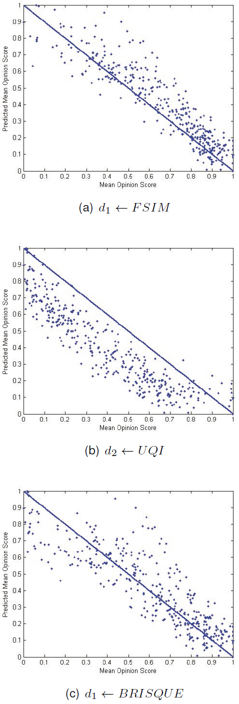
Fig. 7 MOS vs MOSp (both normalized). MOSp is predicted by (a) d1 using FSIM, (b) d2 using UQI, and (c) d1 using BRISQUE
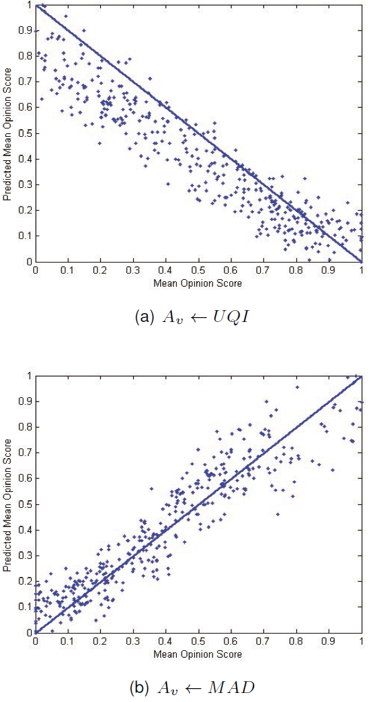

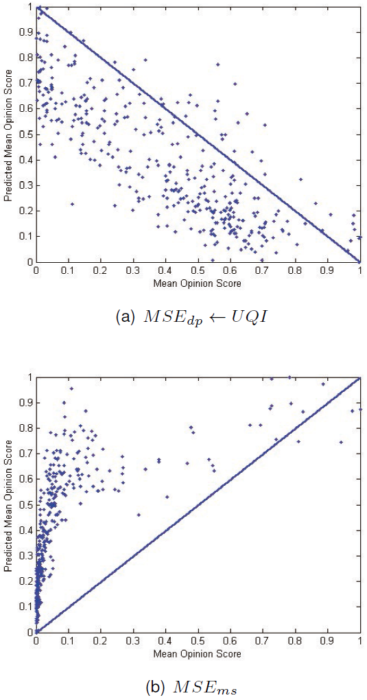

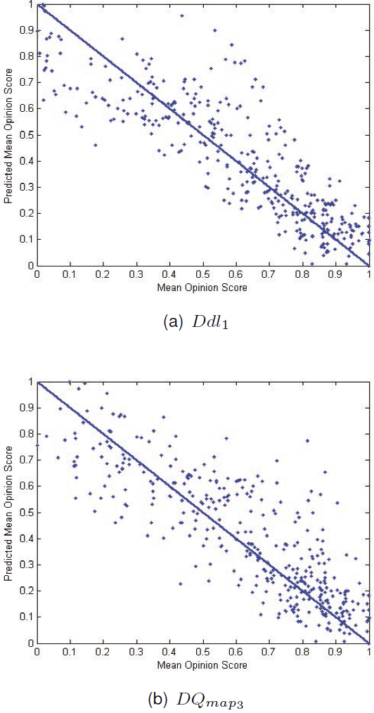
Table 4 Overall performance of the metrics proposed by [3] in predicting perceived stereoscopic image quality: Linear Correlation Coefficient (LCC), Spearman's Rank Ordered Correlation Coefficient (SROCC), Kendall's Rank Ordered Correlation Coefficient (KROCC) and Root Mean Squared Error (RMSE)
| Distortion | SIQA | 2DIQA | PM | Value |
|---|---|---|---|---|
| ALL | d1 | FSIM | LCC | 0.9169 |
| d2 | UQI | SROCC | 0.9335 | |
| d2 | UQI | KROCC | 0.7659 | |
| d1 | BRISQUE | RMSE | 0.1485 | |
| JP2K | d2 | UQI | LCC | 0.9304 |
| d2 | UQI | SROCC | 0.9104 | |
| d2 | UQI | KROCC | 0.7405 | |
| d3 | MSE | RMSE | 0.1583 | |
| JPEG | d2 | UQI | LCC | 0.7620 |
| d2 | UQI | SROCC | 0.7268 | |
| d2 | UQI | KROCC | 0.5212 | |
| d3 | MSE | RMSE | 0.1080 | |
| WN | Ddl1 | none | LCC | 0.9330 |
| d1 | MSSIM | SROCC | 0.9403 | |
| d1 | MSE | KROCC | 0.7861 | |
| d1 | BRISQUE | RMSE | 0.1001 | |
| Blur | d2 | UQI | LCC | 0.9558 |
| d2 | UQI | SROCC | 0.9306 | |
| d1 | MSSIM | KROCC | 0.7758 | |
| d1 | BRISQUE | RMSE | 0.1442 | |
| FF | d2 | UQI | LCC | 0.8549 |
| d2 | UQI | SROCC | 0.8162 | |
| d2 | UQI | KROCC | 0.6245 | |
| d2 | NR-PSNR | RMSE | 0.1116 |
Table 5 Overall performance of the metrics proposed by [7] in predicting perceived stereoscopic image quality: Linear Correlation Coefficient (LCC), Spearman's Rank Ordered Correlation Coefficient (SROCC), Kendall's Rank Ordered Correlation Coefficient (KROCC) and Root Mean Squared Error (RMSE)
| Distortion | SIQA | 2DIQA | PM | Value |
|---|---|---|---|---|
| ALL | Av | UQI | LCC | 0.9371 |
| Av | MAD | SROCC | 0.9394 | |
| Av | MAD | KROCC | 0.7772 | |
| Av | MAD | RMSE | 0.0732 | |
| JP2K | Av | UQI | LCC | 0.9441 |
| Av | MAD | SROCC | 0.9247 | |
| Av | MAD | KROCC | 0.7663 | |
| Av | MAD | RMSE | 0.0630 | |
| JPEG | Av | MAD | LCC | 0.7686 |
| Va | MAD | SROCC | 0.7388 | |
| Va | MAD | KROCC | 0.5408 | |
| Av | MAD | RMSE | 0.0529 | |
| WN | Av | MAD | LCC | 0.9523 |
| Av | MAD | SROCC | 0.9497 | |
| Av | MAD | KROCC | 0.8044 | |
| Av | MAD | RMSE | 0.0805 | |
| Blur | Av | MAD | LCC | 0.9660 |
| Av | MAD | SROCC | 0.9537 | |
| Av | MAD | KROCC | 0.8362 | |
| Va | BIQI | RMSE | 0.0759 | |
| FF | Av | UQI | LCC | 0.8787 |
| Av | UQI | SROCC | 0.8328 | |
| Av | UQI | KROCC | 0.6447 | |
| Av | MAD | RMSE | 0.0861 |
Table 6 Overall performance of the metric proposed by [16] in predicting perceived stereoscopic image quality: Linear Correlation Coefficient (LCC), Spearman's Rank Ordered Correlation Coefficient (SROCC), Kendall's Rank Ordered Correlation Coefficient (KROCC) and Root Mean Squared Error (RMSE)
| Distortion | SIQA | 2DIQA | PM | Value |
|---|---|---|---|---|
| ALL | PSNRedge | NCC | LCC | 0.5772 |
| PSNRedge | VIFP | SROCC | 0.7976 | |
| PSNRedge | VIFP | KROCC | 0.5958 | |
| PSNRedge | AD | RMSE | 0.2084 | |
| JP2K | PSNRedge | NQM | LCC | 0.7749 |
| PSNRedge | NQM | SROCC | 0.8045 | |
| PSNRedge | NQM | KROCC | 0.6082 | |
| PSNRedge | SC | RMSE | 0.1641 | |
| JPEG | PSNRedge | NQM | LCC | 0.4916 |
| PSNRedge | NQM | SROCC | 0.4860 | |
| PSNRedge | NQM | KROCC | 0.3376 | |
| PSNRedge | VSNR | RMSE | 0.0913 | |
| WN | PSNRedge | NQM | LCC | 0.7999 |
| PSNRedge | VIFP | SROCC | 0.8616 | |
| PSNRedge | VIFP | KROCC | 0.6652 | |
| PSNRedge | NAE | RMSE | 0.2084 | |
| Blur | PSNRedge | SSIM | LCC | 0.8114 |
| PSNRedge | NQM | SROCC | 0.8385 | |
| PSNRedge | NQM | KROCC | 0.6646 | |
| PSNRedge | NAE | RMSE | 0.1156 | |
| FF | PSNRedge | NCC | LCC | 0.7738 |
| PSNRedge | NCC | SROCC | 0.7022 | |
| PSNRedge | NCC | KROCC | 0.5188 | |
| PSNRedge | AD | RMSE | 0.1449 |
Table 7 Overall performance of the metrics proposed by [21] in predicting perceived stereoscopic image quality: Linear Correlation Coefficient (LCC), Spearman's Rank Ordered Correlation Coefficient (SROCC), Kendall's Rank Ordered Correlation Coefficient (KROCC) and Root Mean Squared Error (RMSE)
| Distortion | SIQA | 2DIQA | PM | Value |
|---|---|---|---|---|
| ALL | MSEdp | UQI | LCC | 0.7962 |
| MSEms | none | SROCC | 0.8952 | |
| MSEms | none | KROCC | 0.7022 | |
| MSEdp | BIQI | RMSE | 0.1754 | |
| JP2K | MSEdp | UQI | LCC | 0.8512 |
| MSEms | none | SROCC | 0.8608 | |
| MSEms | none | KROCC | 0.6620 | |
| MSEdp | MSE | RMSE | 0.1583 | |
| JPEG | MSEdp | UQI | LCC | 0.5769 |
| MSEdp | UQI | SROCC | 0.5779 | |
| MSEdp | UQI | KROCC | 0.4085 | |
| MSEdp | VSNR | RMSE | 0.1031 | |
| WN | MSEdp | UQI | LCC | 0.8832 |
| MSEms | none | SROCC | 0.9310 | |
| MSEms | none | KROCC | 0.7665 | |
| MSEdp | BIQI | RMSE | 0.1130 | |
| Blur | MSEdp | FSIM | LCC | 0.8531 |
| MSEms | none | SROCC | 0.9318 | |
| MSEms | none | KROCC | 0.7717 | |
| MSEdp | BPSNR | RMSE | 0.2192 | |
| FF | MSEdp | PSNRHVSM | LCC | 0.7244 |
| MSEms | none | SROCC | 0.6859 | |
| MSEms | none | KROCC | 0.4998 | |
| MSEdp | JQS | RMSE | 0.1766 |
Table 8 Overall performance of the metrics proposed by [49] in predicting perceived 3D image quality: Linear Correlation Coefficient (LCC), Spearman's Rank Ordered Correlation Coefficient (SROCC), Kendall's Rank Ordered Correlation Coefficient (KROCC) and Root Mean Squared Error (RMSE)
| Distortion | SIQA | 2DIQA | PM | Value |
|---|---|---|---|---|
| ALL | YouDMOSp | UQI | LCC | 0.9371 |
| YouDMOSp | UQI | SROCC | 0.9372 | |
| YouDMOSp | UQI | KROCC | 0.7722 | |
| DQmap2 | none | RMSE | 0.1289 | |
| JP2K | YouDMOSp | UQI | LCC | 0.9441 |
| YouDMOSp | UQI | SROCC | 0.9095 | |
| YouDMOSp | UQI | KROCC | 0.7405 | |
| DQmap2 | none | RMSE | 0.0961 | |
| JPEG | YouDMOSp | UQI | LCC | 0.7678 |
| YouDMOSp | UQI | SROCC | 0.7383 | |
| YouDMOSp | UQI | KROCC | 0.5358 | |
| DQmap2 | none | RMSE | 0.0742 | |
| WN | YouDMOSp | SSIM | LCC | 0.9326 |
| OQ | MSSIM | SROCC | 0.9425 | |
| OQ | MSSIM | KROCC | 0.7911 | |
| YouDMOSp | NAE | RMSE | 0.1237 | |
| Blur | YouDMOSp | UQI | LCC | 0.9517 |
| YouDMOSp | MSSIM | SROCC | 0.9282 | |
| YouDMOSp | AD | KROCC | 0.7818 | |
| OQ | VSNR | RMSE | 0.2097 | |
| FF | YouDMOSp | UQI | LCC | 0.8787 |
| YouDMOSp | UQI | SROCC | 0.8328 | |
| YouDMOSp | UQI | KROCC | 0.6447 | |
| DQmap2 | none | RMSE | 0.1498 |
Table 9 Overall performance of the Stereoscopic Metrics in predicting perceived stereoscopic image quality: Linear Correlation Coefficient (LCC), Spearman's Rank Ordered Correlation Coefficient (SROCC), Kendall's Rank Ordered Correlation Coefficient (KROCC) and Root Mean Squared Error (RMSE)
| Distortion | SIQA | PM | Value |
|---|---|---|---|
| ALL | Ddl1 | LCC | 0.8629 |
| MSEms | SROCC | 0.8952 | |
| MSEms | KROCC | 0.7022 | |
| DQmap2 | RMSE | 0.1289 | |
| JP2K | DQmap3 | LCC | 0.8604 |
| DQmap3 | SROCC | 0.8638 | |
| MSEms | KROCC | 0.6620 | |
| DQmap2 | RMSE | 0.0961 | |
| JPEG | DQmap3 | LCC | 0.5750 |
| DQmap3 | SROCC | 0.5439 | |
| DQmap3 | KROCC | 0.3806 | |
| DQmap2 | RMSE | 0.0742 | |
| WN | Ddl1 | LCC | 0.9330 |
| Ddl1 | SROCC | 0.9380 | |
| Ddl1 | KROCC | 0.7829 | |
| ODDM4 | RMSE | 0.1079 | |
| Blur | Ddl1 | LCC | 0.9056 |
| MSEms | SROCC | 0.9318 | |
| MSEms | KROCC | 0.7717 | |
| ODDM4 | RMSE | 0.1304 | |
| FF | ODDM4 | LCC | 0.7540 |
| ODDM4 | SROCC | 0.7734 | |
| ODDM4 | KROCC | 0.5783 | |
| ODDM4 | RMSE | 0.1490 |
Table 10 Overall performance across SIQA-SET in predicting perceived 3D image quality: Linear Correlation Coefficient (LCC), Spearman's Rank Ordered Correlation Coefficient (SROCC), Kendall's Rank Ordered Correlation Coefficient (KROCC) and Root Mean Squared Error (RMSE)
| Distortion | SIQA | 2DIQA | PM | Value |
|---|---|---|---|---|
| ALL | YouDMOSp | UQI | LCC | 0.9371 |
| Av | MAD | SROCC | 0.9394 | |
| Av | MAD | KROCC | 0.7772 | |
| Av | MAD | RMSE | 0.0732 | |
| JP2K | YouDMOSp | UQI | LCC | 0.9441 |
| Av | MAD | SROCC | 0.9247 | |
| Av | MAD | KROCC | 0.7663 | |
| Av | MAD | RMSE | 0.0630 | |
| JPEG | Av | MAD | LCC | 0.7686 |
| Va | MAD | SROCC | 0.7388 | |
| Va | MAD | KROCC | 0.5408 | |
| Av | MAD | RMSE | 0.0529 | |
| WN | Av | MAD | LCC | 0.9523 |
| Av | MAD | SROCC | 0.9497 | |
| Av | MAD | KROCC | 0.8044 | |
| Av | MAD | RMSE | 0.0805 | |
| Blur | Av | MAD | LCC | 0.9660 |
| Av | MAD | SROCC | 0.9537 | |
| Av | MAD | KROCC | 0.8362 | |
| Va | BIQI | RMSE | 0.0759 | |
| FF | Av | UQI | LCC | 0.8787 |
| Av | UQI | SROCC | 0.8328 | |
| Av | UQI | KROCC | 0.6447 | |
| Av | MAD | RMSE | 0.0861 |
Table 11 Performance across SIQA-SET in predicting perceived stereoscopic image quality: Linear Correlation Coefficient (LCC). Bold indicates the best metric, while italics the second best
| Author | SIQA | 2DIQA | JP2K | JPEG | WN | Blur | FF | ALL |
|---|---|---|---|---|---|---|---|---|
| Benoit et al.[3] | d1 | FSIM | 0.9119 | 0.6259 | 0.9307 | 0.9358 | 0.7834 | 0.9169 |
| Bosc et al.[5] | Qs | none | 0.0259 | 0.1563 | 0.8866 | 0.1853 | 0.0882 | 0.4115 |
| Campisi et al.[7] | Av | UQI | 0.9441 | 0.7678 | 0.9199 | 0.9517 | 0.8787 | 0.9371 |
| Gu et al.[15] | ODDM4 | none | 0.7728 | 0.4461 | 0.9223 | 0.7024 | 0.7540 | 0.7460 |
| Hewage et al.[16] | PSNRedge | NCC | 0.6737 | 0.3293 | 0.7997 | 0.8027 | 0.7738 | 0.5772 |
| Jin et al.[21] | MSEdp | UQI | 0.8512 | 0.5769 | 0.8832 | 0.8523 | 0.6327 | 0.7962 |
| Joveluro et al.[22] | PQM3D | none | 0.1393 | 0.2415 | 0.8477 | 0.0444 | 0.1765 | 0.4790 |
| Mao et al.[24] | Qmao | none | 0.7189 | 0.1290 | 0.7701 | 0.7527 | 0.4413 | 0.7082 |
| Yang et al.[48] | IQA | none | 0.7665 | 0.1187 | 0.9244 | 0.7690 | 0.6993 | 0.7002 |
| You et al.[49] | YouDMOSp | UQI | 0.9441 | 0.7678 | 0.9199 | 0.9517 | 0.8787 | 0.9371 |
Table 12 Performance across SIQA-SET in predicting perceived stereoscopic image quality: Spearman's Rank Ordered Correlation Coefficient (SROCC). Bold indicates the best metric, while italics the second best
| Author | SIQA | 2DIQA | JP2K | JPEG | WN | Blur | FF | ALL |
|---|---|---|---|---|---|---|---|---|
| Benoit et al.[3] | d2 | UQI | 0.9104 | 0.7268 | 0.9248 | 0.9306 | 0.8162 | 0.9335 |
| Campisi et al.[7] | Av | MAD | 0.9247 | 0.7364 | 0.9497 | 0.9537 | 0.7720 | 0.9394 |
| Gorley et al.[14] | SBLC | none | 0.6744 | 0.4431 | 0.6219 | 0.6229 | 0.2133 | 0.5963 |
| Gu et al.[15] | ODDM4 | none | 0.8131 | 0.4202 | 0.9206 | 0.6577 | 0.7734 | 0.7223 |
| Hewage et al.[16] | PSNRedge | VIFP | 0.7802 | 0.2360 | 0.8616 | 0.7958 | 0.5027 | 0.7976 |
| Jin et al.[21] | MSEms | AD | 0.8608 | 0.4484 | 0.9310 | 0.9318 | 0.6859 | 0.8952 |
| Joveluro et al.[22] | PQM3D | none | 0.0239 | 0.1329 | 0.9167 | 0.1398 | 0.3360 | 0.2667 |
| Mao et al.[24] | Qmao | none | 0.7460 | 0.1629 | 0.7790 | 0.6279 | 0.3599 | 0.7253 |
| Yang et al.[48] | IQA | none | 0.7993 | 0.1212 | 0.9316 | 0.9020 | 0.5875 | 0.8340 |
| You et al.[49] | YouDMOSp | UQI | 0.9095 | 0.7383 | 0.9255 | 0.9252 | 0.8328 | 0.9372 |
Table 13 Performance across SIQA-SET in predicting perceived stereoscopic image quality: Kendall's Rank Ordered Correlation Coefficient (KROCC). Bold indicates the best metric, while italics the second best
| Author | SIQA | 2DIQA | JP2K | JPEG | WN | Blur | FF | ALL |
|---|---|---|---|---|---|---|---|---|
| Benoit et al.[3] | d2 | UQI | 0.7405 | 0.5212 | 0.7570 | 0.7697 | 0.6245 | 0.7659 |
| Campisi et al.[7] | Av | MAD | 0.7663 | 0.5377 | 0.8044 | 0.8362 | 0.5909 | 0.7772 |
| Gorley et al.[14] | SBLC | none | 0.4608 | 0.3065 | 0.4468 | 0.4141 | 0.1510 | 0.4201 |
| Gu et al.[15] | ODDM4 | none | 0.6089 | 0.2666 | 0.7456 | 0.5071 | 0.5783 | 0.5284 |
| Hewage et al.[16] | PSNRedge | VIFP | 0.5899 | 0.1596 | 0.6652 | 0.6222 | 0.3694 | 0.5958 |
| Jin et al.[21] | MSEms | AD | 0.6620 | 0.2869 | 0.7665 | 0.7717 | 0.4998 | 0.7022 |
| Joveluro et al.[22] | PQM3D | none | 0.0152 | 0.0893 | 0.7473 | 0.0929 | 0.2263 | 0.1869 |
| Mao et al.[24] | Qmao | none | 0.5418 | 0.1216 | 0.5791 | 0.4525 | 0.2535 | 0.5294 |
| Yang et al.[48] | IQA | none | 0.5918 | 0.0735 | 0.7665 | 0.7333 | 0.4168 | 0.6296 |
| You et al.[49] | YouDMOSp | UQI | 0.7405 | 0.5358 | 0.7570 | 0.7636 | 0.6447 | 0.7722 |
Table 14 Performance across SIQA-SET in predicting perceived stereoscopic image quality: Root Mean Squared Error (RMSE). Bold indicates the best metric, while italics the second best
| Author | SIQA | 2DIQA | JP2K | JPEG | WN | Blur | FF | ALL |
|---|---|---|---|---|---|---|---|---|
| Benoit et al.[3] | d1 | BRISQUE | 0.1935 | 0.1750 | 0.1001 | 0.1442 | 0.1278 | 0.1485 |
| Campisi et al.[7] | Av | MAD | 0.0630 | 0.0529 | 0.0805 | 0.0919 | 0.0861 | 0.0732 |
| Gorley et al.[14] | SBLC | none | 0.2980 | 0.1923 | 0.4733 | 0.3872 | 0.5295 | 0.3750 |
| Gu et al.[15] | ODDM4 | none | 0.1041 | 0.1654 | 0.1079 | 0.1304 | 0.1490 | 0.1315 |
| Hewage et al.[16] | PSNRedge | AD | 0.1995 | 0.1875 | 0.2949 | 0.2203 | 0.1449 | 0.2084 |
| Jin et al.[21] | MSEdp | BIQI | 0.1840 | 0.1726 | 0.1130 | 0.2714 | 0.1778 | 0.1754 |
| Mao et al.[24] | Qmao | none | 0.3899 | 0.4327 | 0.3921 | 0.3730 | 0.3014 | 0.3783 |
| Shen et al.[38] | HDPSNR | none | 0.2035 | 0.2237 | 0.2981 | 0.2162 | 0.2549 | 0.2415 |
| Yang et al.[48] | IQA | none | 0.2081 | 0.0931 | 0.4136 | 0.3473 | 0.4275 | 0.2932 |
| You et al.[49] | DQmap2 | VSNR | 0.0961 | 0.0742 | 0.1273 | 0.2506 | 0.1498 | 0.1289 |
5.1 Metrics based on 2DIQA
In this subsection, we expose the results not only of SIQA based on 2DIQA but also of certain authors that propose more than one SIQA. We use ← to refer that we applied a certain 2DIQA algorithm into a SIQA.
— d1, d2, d3 and Ddl1. We obtain 88 metrics after combing d1, d2, and d3 with 2DIQA-SET in addition to perform Ddl1. If we correlate these 88 variations with the all 365 images of the LIVE 3D image database we obtain the results of the Table 4, which shows that the best linear correlation is obtained by d1 ← FSIM (91.69%), see also Figure 7(a). While d 2 ← UQI is the best ranking metric, since both in SROCC and KROCC, it obtains the best correlation with the human observers. Also, based on the results of d1 ← BRISQUE is clear that for the set of distortions considered, this metric is the most accurate. Considering just distortions in the field of image compression, JPEG2000 and JPEG, we can highlight d2 ← UQI is the best metric in either linear or rank (not-linear) correlation.
Figures 7(b) and 7(c) depict the scatter plots both for d2 ← UQI and d1 ← BRISQUE, where we show the dispersion of the results obtained by these metrics.
— Av and Va. We could evaluate 58 variations of these two algorithms and we obtain the results of the Table 5, which shows that the best linear correlation is obtained by Av ← UQI (93.94%), see also Figure 8(a). In Figure 8(b), Av ← MAD is the best ranking metric, since both in SROCC and KROCC it obtains the best correlation with the human observers, in addition, this metric is the most accurate since it obtained the less RMSE.
For JPEG2000 Distortion, Av ← MAD is the best ranking metric, i.e. to average right and left MAD qualities, if we change the weighted parameters of the stereo-pair, namely Va ← MAD, we get the best ranking metric for JPEG distortion.
— PSNRedge. Despite our modification of this algorithm, which included using not only PSNR but also any metric of the 2DIQA-SET (Table 6), we obtain that PSNRedge ← NCC is slightly correlated with HVS, Figure 9, which incidentally is the best metric in terms of linear correlation. Furthermore, PSNRedge ← VIFP is the best overall ranking metric with about 15 percent less correlated with HVS than other metrics described previously.
— MSEms, and MSEdp. From Table 7, when we average individual qualities of right and left depth maps, i.e. MSEdp, it obtained the best results for LCC (Fig. 10(a)) and RMSE in all distortions. In this way, MSEdp ← UQI is highly linear correlated with the opinion of observers for the included image compression distortions. The ranking obtained by MSEms is better correlated with HVS than the one gotten by MSEdp, across all kind of distortions of LIVE 3D.
Figure 10(b) shows that not always an excellent ranking means accuracy of results, even the difference between estimations is important, MSEms ranks the 90% of the results (SROCC) in the same order that an observer could do it.
— YouDMOSp, OQ, DQmap1, DQmap2, and DQmap3 . UQI measures the degree of linear correlation between original and distorted signals [42], when it is combined with a nonlinear regression of average of the quality of single views, using Equation 13, we found the best results in all distortions, except White Noise.
The scatter plot of Figure 11(a) depicts that YouDMOSp results tend to be more concentrated along perfect correlation. In brief, Table 8 shows that YouDMOSp ← UQI performs better results in terms of any kind of correlation coefficient but it is not as accurate as DQmap2 and viceversa, which is why in Figure 11(b) the results of DQmap2 are more dispersed and its results are closer to the perfect result than YouDMOSp results.
5.2 Stereoscopic Metrics
In this subsection, we sketch only the results of metrics that do are not based on a normal metric or they just are based in one feature of a certain normal image quality assessment.
Table 9 just contains the results of all stereoscopic metrics exposed in subsection 4.2. Where Ddl1 linear correlates in 86.29%, Figure 12(a), being the assessment that estimates the best Linear Correlation. Furthermore, MSEms is the best ranked metric obtaining the best results both in SROCC and KROCC with 89.52% and 70.22%, respectively.
Also, DQmap2 is the most precise stereoscopic assessment for all whole of considered noises and image compression noises such as JPEG2000 and JPEG distortions.
Taking in to account only noises produced by a image compression coder, DQmap3 is best metric in LCC and SROCC. Figure 12(b) depicts dispersion of the 365 results of DQmap3.
5.3 ALL SIQA-SET
Regarding the overall experimental results, Table 10 depicts the performance of all SIQA of the SIQA-SET exposed in section 4.
Thus, Figure 11(a) shows the metric YouDMOSp ← UQI, this assessment linear correlates in 93.71% and obtains the best Linear Correlation.
Furthermore, the best ranked metric is Av ← MAD, because it is best correlated both in SROCC and KROCC with 93.94% and 77.72%, respectively.
Also, we can say that Av ← MAD is the most precise algorithm for all set of distortions considered and JPEG2000 and JPEG noises. Regarding only these image compression distortions, Av ← MAD is the best ranking metric, i.e. to average right and left MAD qualities, if we change the weighted parameters of the stereo-pair, namely Va ← MAD, we get the best ranking metric for JPEG distortion.
In this paper we have presented several metrics (280) for gauging the quality of a stereo-pair intended for researchers interested in stereoscopic coding, visual discomfort or stereoscopic displaying. These researchers could want to found the best metric taking into account a certain respond in a certain distortion, for example.
The selected metric could be the best overall measure, which does not mean it would obtain the best results in all individual distortions. For those researchers who are interested in knowing the behavior of the top-ten overall SIQA-SET, we propose Tables 11 to 14, which were made considering the following aspects:
— Each Table represents only one Performance Measure, either LCC, SROCC, KROCC, or RMSE.
— In order to rank the 17 authors, we just chose the best metric (across all images in LIVE 3D) for those authors who proposed more than one SIQA.
— Regards overall performance, we eliminated the seven metrics that obtained the worst effects.
— Once we obtained the top-ten we indicated with Bold text the best metric, while with italic text the second best metric.
— Finally, we sorted alphabetically the top-ten by author name.
From Table 11 Av ← UQI (Fig. 8(a)) and YouDMOSp ← UQI (Fig. 11(a)) obtained the best results in linear correlation coefficient not only in overall performance (93.71%) but also in all individual distortions, except in White Noise. For White Noise d1 ← FSIM (Fig. 7(a)) is the best metric with 93.07%.
Table 12 shows the performance across SIQA-SET in estimating subjective 3D/stereoscopic image quality using SROCC. Where Av ← MAD (Fig. 8(b)) obtained the best results in overall performance (93.94%), JPEG2000 (92.47%), White Noise (94.97%), and Gaussian Blur (95.37%). While YouDMOSp ← UQI (Fig. 11(a)) got the best results in JPEG (73.83%), and Fast Fading distortion (83.28%).
From Table 13 Av - MAD (Fig. 8(b)) obtained the best results in linear correlation coefficient not only in overall performance (77.72%) but also in all individual distortions, except in Fast Fading distortion. For Fast Fading distortion YouDMOSp ← UQI (Fig. 11(a)) is the best metric with 64.47%.
Table 14 shows the performance across SIQA-SET in prediction of the perceived stereoscopic image quality using Root Mean Squared Error. Where Av ←MAD (Fig. 8(b)) obtained the best results not only in overall performance (0.0732), but also in JPEG2000 (0.0630), JPEG (0.0529), White Noise (0.0805), Gaussian Blur (0.0919), and Fast Fading distortion (0.0861).
6 Conclusions and Future Work
This paper describes 27 algorithms SIQA exposed by 17 authors, summarizing the research made in 3D/stereoscopic image quality field in the recent years. Nine metrics of this SIQA-SET can be combined with any 2DIQA, then they were separated from rest. These metrics were defined as Metrics based on 2DIQA and they were tested with 29 2DIQA, having a total of 262. Thus, we considered that the remaining 18 metrics were grouped as Stereoscopic Metrics.
For Metrics based on 2DIQA YouDMOSp using UQI got the best linear correlation, 94%, with the opinion of an observer, same percentage obtained by Av using MAD but employing a no-linear correlation. For Stereoscopic Metrics, Ddl1 got the best linear correlation (86%) with the opinion of an observer, whereas in the 89% MSEdp similarly ranked as a human observer, if no-linear correlation is employed.
The difference between YouDMOSp and Av is that the first use a nonlinear regression function of the average of certain 2DIQA metric while the latter is just the mean of one of 29 2DIQA applied to stereo-pair, in this way YouDMOSp with UQI is linearly better than Av with UQI for just 0.000611%.
So, our results of these 27 algorithms in the field of SIQA could lead to conclude that Metrics based on 2DIQA can assess the perceptual quality of third dimensional or stereoscopic images. The implication of results of the presented research should be considered with caution, since the first matter to observe is that the majority of the Stereoscopic Metrics are only adaptations of 2DIQA, which add some features such as depth variances from the disparity map, for instance. Any perceptual feature is included in the manner that this disparity information is taken, namely any algorithm incorporates disparity masking.
It is important to realize that observers employed not only in LIVE 3D but also in MMSPG or FISE image databases judge the stereoscopic image quality watching some slices, apparently separated, of a 2D scenario, which is a disadvantage for the Stereoscopic Metrics. Also, another disadvantage for Stereoscopic Metrics is that the distortions in LIVE 3D image database are not designed or applied stereoscopically, since they separately distorted the left and right images.
Some distortions that LIVE 3D image database considers, such as Gaussian Blur and Additive White Gaussian Noise, are global distortions and therefore, they would not affect too much the perception of depth. Not only Metrics based on 2DIQA correlates extremely well with these distortions but also some Stereoscopic Metrics do it well, such as d1 or MSEdp. However for those distortions with localized artifacts, the performance both of Metrics based on 2DIQA and Stereoscopic Metrics is lower, especially for the local blocking artifacts caused by a JPEG compression. Furthermore, some irregularities in terms of the depth map appear when localized distortions are evaluating, which is why the presented state-of-the-art SIQA-SET does not correlate well. For JPEG compression distortion, the performance of YouDMOSp and Av is unexpectedly good in spite of being dependant functions on a monoscopic image quality.
If we take in to account that Stereoscopic Metrics are simple designs somehow based on a certain 2DIQA, we also can realize that the gap between Stereoscopic Metrics and Metrics based on 2DIQA can be filled proposing assessments with some features of the best correlated metrics.

