1 Introduction

According to the foundations of the quantum mechanics, the complete description of a quantum system relies on the knowledge of the state vector V> that belongs to the space states ^[5]. However, it is difficult to extract, in a transparent manner, the most relevant physical insights of a quantum system through the single analysis of its vector state. Fortunately, several useful representations can demystify its abstract nature, among them we find the Wigner function. It is primordially appropriated to discuss the connection between the classical and the quantum domain ^[15].

The initial emergence of the field Wigner function in cavities has become increasingly important as fundamental Quantum question has received a renewed attention and that demanded of a handy theoretical, numerical and experimental tool able, as the Wigner function, to express its analysis. This is particularly important in composite quantum systems ^[11], where its complexity limits quite frequently our ability to provide fully solvable results.

In those systems, the Wigner function becomes far too complex to be solved analytically and the need to have a fully numerical approach is required. The aim of this work is to introduce a numerical approach that can explore from its basics.

Several equivalent definitions allow the computation of the Wigner function. If it is known the quantum system stationary wave function 4> (x), we can easily compute the Wigner function through the following expression ^[15]:

An alternative and equivalent way to compute the Wigner function is through ^[3]:

Let us notice that while the equation 1 is valid for a system described by the wave function ϕ(x), the equation 2 is of more general application because applies to a quantum system described by the density operator ρ.

Maybe, the most widely discussed model in quantum optics is the Jaynes-Cummings Model (JCM), which in its simplest form describes the interactions between a two-level atom and the quantized field in a perfect cavity ^[10]. The analysis of the field Wigner function in this model is a standard tool to inquire on the properties of the cavity quantum field. To compute the JCM Wigner function, it has been proposed the factorization of JCM the wave function as:

is a key step in the discussions of the analytical time-dependent JCM Wigner function. The limitation of the equation 3 is its validity only for fields described by a vector state, and it is desirable to generalize such expression to take into account a density matrix formalism. Such a handy factorization has been possible through the assumption of exact atom-field resonance ^[6].

In the equation 3, the first term is related to the ground state and the second one to the excited state. An analysis without those assumptions becomes quite a formidable task, which implicitly makes desirable numerical strategies that could provide an efficient analysis to more complex cases. This numerical perspective is the motivation of our didactic examination of the JCM Wigner function as a convenient example, which can be extended to discuss many other problems.

The starting point of our discussion will be the equation 2. The computational implementation of the quantum operators, which appear in such equation, becomes viable by taking advantage of the modern software available for the matrix management. The quantum practitioner, which often finds these complex operator expressions, will appreciate it to explore these techniques in many other problems further.

2 The Harmonic Oscillator Wigner Function

The Harmonic Oscillator (HO) is one of the most widely used models in many areas of physics. The quantum version of this model is the mathematical tool to describe the quantum field inside a perfect cavity. Therefore, before inquiring into the JCM cavity field Wigner function, it is convenient to briefly describe the quantum harmonic oscillator and to show the the expressions of its time-dependent Wigner function. The Hamiltonian of the quantum harmonic oscillator is:

HHO=ħωa†a+12, (4)

where its frequency is given by ω and the rising and lowering operators are provided by a† and a respectively, and their properties have a vast literature.

There are quantum states expressed in terms of a and a† , as the mathematical tool to describe the quantum field in cavities. The Fock state n is defined through the eigenvalue relation a†an=nn, where n denotes an integer number. The Fock states are known for having a well-defined number of quanta and for not having a classical counterpart. These states are particularly relevant since they allow a discrete representation of quantum states and operators, which is a convenient way for its numerical implementation. The coherent states, introduced by Glauber ^[7], are defined as the eigenstate of the annihilation operator aα=αα, where α is, in general, a complex number. They have the closest classical-like behavior, and they describe the laser beam light accurately.

The HO propagator is just the exponential of the Hamiltonian exp-iHt/ħ:

UHOt=exp⁡-iωa†at. (5)

Moreover, the HO state at an arbitrary time t is:

ϕt=UHOtϕ0. (6)

Two typical examples of propagating an initial state are the Fock state n , which at t acquires only a phase factor e-inωtn. On the other hand, if the HO initially is a coherent state, the state becomes αe-iωt. The corresponding analytical expression of the Wigner function is:

Wα,α*=2-1ne-4α2Ln2α2, (7)

for a Fock state. In equation (1.7) n denotes the HO number of quanta, and L_n(x) denotes the nth-order Laguerre polynomial. Notice that this Wigner function is time-independent because in this case the density matrix does not depend explicitly on time, see Fig. 1. The Wigner function of a coherent state is given by:

Wα,α*=2e-α-α0t2. (8)

Figure 1 Numerical evaluation of the Fock state Wigner function of a harmonic oscillator prepared with 9 photons. This Wigner function has negative zones, indicating it is a non-classical state and it is time-independent because the evolution of the Fock state is determined only by a phase factor 

The equation 8 describes a clockwise rotating two-dimensional Gaussian function in the complex plane defined by α, which is centered at α0t. Both didactic examples 7 and 8, as well the Wigner function of other remarkable states, are well-known and are reported in te literature ^[14].Despite the simplicity of the analytical expressions 7 and 8, the computations are lengthy, even under this simple Hamiltonian.

3 The Jaynes-Cummings Model

The Jaynes-Cummings Model (JCM) ^[10] is one of the most notorious physical models to accurately describe the interactions between the quantized field in a one-dimensional perfect cavity of frequency ω and a Two-Level Atom (TLA) with atomic transition frequency w₀ . The strength of such interactions are provided by the coupling constant A. The JCM Hamiltonian is:

The above Hamiltonian was obtained under Rotating Wave Approximation (RWA). Just like we anticipated, the operator a describes the cavity mode, and satisfies the usual Bosonic operators commutation rule a†,a=1 . On the other hand, the atomic rising σ+=1-1 and lowering σ-=-11 operators govern the transitions between the atomic excited 1 and ground state -1 They are related to the atomic inversion operator through the commutation rule σz=σ+,σ- .

There are several outstanding mathematical properties of this model. One of them is the existence of motion constants. They are the total number of excitation and the interchange constant ^[1], which are given by:

Often the computation of JCM analytical expressions relies on the knowledge of these constants. Furthermore, the technique of finding the motion constants is quite a useful path for solving more complex quantum-electrodynamical systems. The propagator of the JCM is given by:

Another JCM feature is the existence of the so-called dressed states that diagonalize the Hamiltonian, and are given by:

In the equation 12 we are going to choose the Bosonic index n satisfying the condition n > 0. The quantities c_n and s_n are a shorthand notation for cn=cosθn/2 and sn=sinθn/2 , where θ_n is defined through:

The dressed states are a complete base for the JCM. Therefore, a JCM unity operator is the following:

The exact JCM eigenfrequencies are ^[13]:

The total excitation was denoted by N_nm , and it is given by:

where n and m are the eigenvalues of the unperturbed operators a†a and σz respectively.

4 Numerical Implementation of Quantum States and Operators

As we have previously pointed out, the time-dependent cavity field Wigner function computation is a formidable task, even in the absence of atomic interactions. However, the definition given in equation 2, provides quite a convenient manner to numerically perform such a task. For this purpose, we have to recall that the quantum states and operators have computer readable representations. In this matrix formulation of the quantum mechanics, a quantum state is described by a column vector while a quantum operator by a matrix. In general, both of them have complex entries.

4.2 Field Operators and States

Field states and operators also have to be implemented on the computer. The Fock n state, and the operators of annihilation and creation, have an infinite dimension. Therefore, a knowledgeable practitioner has to approximate them. Let us choose a convenient example of truncation at n_max = 5. We have to establish a criterion to obtain an upper bound to describe numerically these operators. Often this upper bound is dictated in terms of state distribution mean number, see Fig. 1. A field described by a Fock state with two photons, n = 2, is approximated by the column vector:

2=00100. (21)

In the same terms, the coherent state can be easily approximated with the following equation:

α=e-α2/2∑n=0nmaxαnn!n, (22)

where α is a complex number. The annihilation operator, in the same terms, has the matrix representation:

α=0001000002000300000400000. (23)

In the same analogous terms, a†=aT due to we have chosen the real representation for the a matrix.

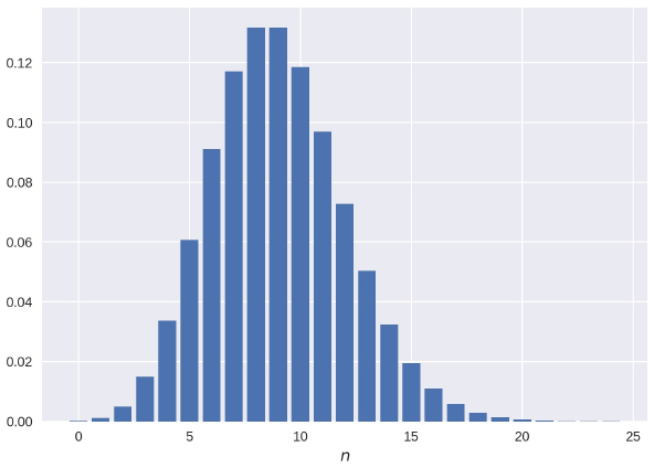
Figure 2 Numerical evaluation of the photon counting probability, i.e., the first 25 diagonal elements of the density matrix α0 α0 . The average number of this distribution has been chosen to be α02=9 . The sum of all these diagonal elements is the total probability and it is numerically equal to 0.999991346873. This tell us that with this number of elements, we have an excellent description of this particular quantum state. 

5 Numerical Computation of the JCM Wigner Function

The matrix formulation of the quantum operators that we provided is intended to describe interacting atom-field systems. However, the definition of Wigner function requires only the density matrix of the field. In addition to the Kronecker product, we have to implement an operation that allows reducing the dimension of the matrix of a composite system to obtain only the density matrix of the field. This operation is called partial trace.

Let us discuss the concept of the trace. Consider an arbitrary base χi that belongs to a Hilbert space H , and also an operator O living in a space denoted by LH . The trace of O is the sum of the diagonal elements in the mentioned base:

where d is the dimension of H . The trace is, in general, a complex quantity and may be taken in another basis which includes those with continuous indices. The JCM density matrix ρJCMt is described in the extended Hilbert space H=HTLA⨂HFIELD . In consequence, we must reduce the dimension of ρJCM by dropping the atomic elements, this procedure is known as partial trace and its denoted by ρFIELD=TrTLAρJCMt . It is implemented through ^[12]:

On the other hand, if we are interested in the atomic density matrix -for instance, to inquire in the Boch vector dynamics-, we can follow an analog definition to obtain the TLA density matrix:

With the knowledge of the density matrix, we can easily implement a routine to compute the Wigner function:

where D(α) is the displacement operator, which is given by:

The numerical implementation of D(α) and eiπa†a can be straightforwardly done in most of the modern software for matrix management. To become computationally more efficient, we can use the cyclic property of the trace and take the trace, by using Fock states, to obtain an expression that requires fewer matrix exponentiations:

The matrix operations involved in the equation 35 makes clear the power of the matrix methods for the computation of the Wigner function.

6 Final Remarks

The numerical techniques here developed can be used to extend easily the results presented in Fig.3. Among these extensions, we can consider the cavity field prepared with other coherence properties. This is done by just changing the initial state of the field ρFIELD . Also, we can explore more complex cases, for instance, the time-dependent Wigner function for the non-resonant JCM, or a TLA prepared in a superposition of excited and ground state. Despite we applied the formalism to the numerical computation of the Wigner function, we also can use it to inquire into other quantities of interest such as expectation values of σ_z, widely known as the atomic inversion.

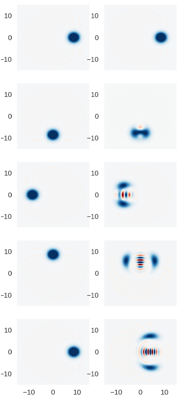
Figure 3 Comparison between the numerical time-dependent Wigner function of a harmonic oscillator (On the left) and the resonant JCM (On the right). In both cases, the initial field is coherent with an average number of photons equal to nine. Consistently with the equation (1.8), the coherent state of the oscillator rotates clockwise keeping its shape. The coherent state in the JCM splits into two contributions, and in the middle, there is exhibit quantum interference that can be interpreted as an atom-field entanglement. Also it is observed a clockwise rotation, which it is reminiscent of the non-interacting part of the JCM Hamiltonian. For this numerical experiment, the TLA was prepared in the excited state 

In the matrix approach here presented, the most relevant source of numerical errors is introduced by the approximated field operators and its posterior exponentiation. To guarantee a good approximation, we have to take the dimension of the approximated field operators n_max large enough; the criterion followed in this work is to select n_max that makes the sum of the diagonal elements very close to 1. Let us recall that in Fig.1 we choose the value 0.999991346873.

There are several matrix management software. Matlab is an excellent option, but also there are free options. For instance numy and scipy, which has the python programming language at its core. These libraries also have capabilities to manage sparse matrices, which can reduce considerably the time of execution of the numerical routines required for the matrix operations in quantum problems.