


 nueva página del texto (beta)
 Inglés (pdf)
 Artículo en XML
 Referencias del artículo
 Enviar artículo por email
 Citado por SciELO
  Similares en
SciELO
Similares en
SciELO 
 Permalink
1 Introduction
Many modern embedded real-time (RT) systems can benefit from today's powerful System-on-Chip multicores (MPSoCs). However, RT task scheduling on multiprocessors is far more challenging than traditional RT scheduling on uniprocessors. Although it is possible to find practical solutions for specific cases, considering thermal restrictions, optimizing energy or dealing with resource sharing are still open questions ([6]). We have been exploring the design of Thermal-Aware RT Schedulers in recent contributions, leveraging control techniques and combining fluid and combinatorial schedulers, taking the most of both approaches ([15]).
On the one hand, fluid schedulers avoid the NP-completeness of a solely combinatorial approach, and allow the use of continuous controllers which make easier to cope with disturbance rejection or to adapt to small parameter variations. On the other hand, the combinatorial approach better matches the nature of the problem, discretizing the fluid schedules to avoid large migrations and context switches.
Testing these kind of schedulers or experimenting with their variations by implementing them on a real system, even on specific evaluation platforms like Litmus-RT ([5]), can be overkilling if we are just performing preliminary explorations of the design space. For this reason, herein we are presenting a novel flexible simulation framework for real time thermal-aware schedulers: TCPN-ThermalSim. It is composed of four main modules, which depend on certain submodules to work.
The first module, which is referred as the configuration module, allows us to introduce the task set according to the three-parameter task model ([7]), or use the UUnifast submodule to generate automatically the task set. It also permits to describe the platform used to execute the task set, composed by the number of CPUs, CPU frequencies and its thermal parameters. The second module is the Kernel simulation, which works over three submodules, where each submodule generates a Timed Continuous Petri Net (TCPN) model that will be merged in order to build a global simulation model. The third module focuses on the scheduler definition, it allows the addition of scheduler algorithms to its analysis. And the last module correspond to the execution of the simulation and present the results as graphs or data in the workspace.
This framework includes out-of-the-box the task, CPU usage and thermal general purpose models reported in [22]. We have included three schedulers: a global EDF scheduler from [1], and other two from our own authorship a RT fluid scheduler ([15]) and a thermal aware RT scheduler ([16]), however the user can define his own scheduler. Sec. 2 provides some background on multiprocessor RT sheduling and Timed Continuous Petri Nets (TCPN), since this formal tool will be used to model the task set, CPU usage and thermal aspects of task execution. Sec. 3 describes the simulation framework architecture and Sec. 4 the user interface. The schedulers included in the framework are described in Sec. 5. Sec. 6 shows a usage example with results, and Sec. 7 presents some conclusions and future work.
2 Background
There are three well-known avenues to leverage multiprocessors for RT scheduling. The partitioned approaches resort to statically allocating tasks to processors. This results into a simple schedulability analysis, since they can use results from RT uniprocessor scheduling. The downside is that this encompasses an NP-hard bin-packing problem and as a consequence, assuring schedulability imposes a maximum CPU utilization bound of 50% or less ([21]).
Global scheduling gets around the problem by dynamically allocating jobs (the periodic tasks' instances) to processors, achieving a 100% utilization bound. Thus, Pfair-based algorithms allocates a new task for execution every time quantum ([26]), which requires that all task parameters are multiples of such a time quantum. The principal inconvenience is that this approach triggers an unfeasible number of preemptions and migrations. By this reason, Deadline partitioning does only take scheduling decisions on the set of all deadlines of all tasks in the system, achieving optimality with fewer preemptions than Pfair([18]).
A third approach mixes static and dynamic allocation. Thus, clustered scheduling statically allocate tasks to clusters of CPUs, but jobs can migrate within their cluster ([8]). Alternatively, semipartitioned scheduling preforms a preliminary static allocation of some tasks over the whole set of available CPUs, allowing the rest of them to migrate ([19]). Recently, [6] and [9] leverage this technique to lowering migrations. In order to test the performance of such schedulers and new ones in early stages, the herein proposed simulation framework is a powerful tool. It is capable to stress schedulers under very realistic conditions, avoiding the effort wasted in adapting the schedulers to actual operating systems and detect from early stages the consequences of a bad heating balance.
When a dynamic thermal balance is a requirement, in order to keep the maximum temperature under control, static allocation techniques are far more restrictive than global approaches. This is the reason why we consider global scheduling, with strategies to minimize preemption and migration like deadline partitioning.
Over the years different real time simulation tools have been proposed, including different features, for example, Cheddar ([25]) is a real time scheduler simulator written in Ada, it handles the multiprocessor case and provides implementations of scheduling, partitioning and analysis algorithms, but their interface is not very user friendly. Another tool is YARTISS ([10]), it evaluates scheduling algorithms by considering overheads or hardware effects, and its design focuses on energy consumption. On the other hand, SimSo ([11]) is a simulation tool that includes different scheduling policies, and takes into account multiple kinds of overheads. All of these tools represent a great aid when developing new algorithms, but none of them is capable of including a thermal model, for this reason we developed TCPN-ThermalSim as a framework capable of developing a thermal analysis of the scheduling algorithms.
Table 1 Software simulation tools comparison
| Framework | Programming language |
Custom Schedulers |
Energy considerations |
Thermal considerations |
|---|---|---|---|---|
| Cheddar | Ada |

|
||
| SimSo | Python |
|
||
| YARTISS | Java |
|
|
|
| TCPN ThermalSim | MATLAB |
|
|
|
Finally, since the proposed framework models tasks and CPUs using Timed Continuous Petri Nets (TCPN), this Section introduces basic definitions concerning Petri nets and continuous Petri nets. An interested reader may also consult [12], [13], [24] to get a deeper insight in the field.
2.1 Discrete Petri Nets
Definition 2.1 A (discrete) Petri net is the 4-tuple N = (P, T, Pre, Post) where P and T are finite disjoint sets of places and transitions, respectively. Pre and Post are |P| × |T| Pre - and Post-incidence matrices, where Pre(i, j) > 0 (resp. Post(i, j) > 0) if there is an arc going from tj to pi (resp. going from pi to tj), otherwise Pre(i, j) = 0 (resp. Post(i, j) = 0).
Definition 2.2 A (discrete) Petri net system is the pair Q =
(N, M) where N is a Petri net and
A transition t∈T is said enabled at the marking
2.2 Continuous and Timed Continuous Petri Nets
Definition 2.3 A continuous Petri Net (ContPN) is a pair
ContPN = (N, m0) where N = (P, T, Pre,
Post) is a Petri net (PN) and
The evolution rule is different from the discrete PN case. In
continuous PN's the firing is not restricted to be integer. A
transition ti in a
ContPN is enabled at
If m is reachable from
m0 by firing the finite sequence
σ
of enabled transitions, then
Definition 2.4 A timed continuous Petri net (TCPN) is a
time-driven continuous-state system described by the tuple (N, λ,
m0) where (N, m0) is a continuous PN and the
vector
Transitions fire according to certain speed, which generally is a function of the
transition rates and the current marking. Such function depends on the semantics
associated to the transitions. Under the infinite server semantics
[23]
the flow through a transition ti
(the transition firing speed) is defined as the product of its rate,
λi , and
enab(ti
, m ), the instantaneous enabling of
the transition, i.e.,
The firing rate matrix is denoted by
A configuration of a TCPN at
m
is a set of arcs
(pi ,
tj ) such that
pi provides the minimum
ratio
The flow through the transitions can be written in vectorial format as
In order to apply a control action to (2), a term u such that 0 ≤ ui ≤ fi (m) is added to every transition ti to indicate that its flow can be reduced. Thus the controlled flow of transition ti becomes wi= fi– ui. Then, the forced state equation is:
2.3 System Definition
The task model accepted by this framework follows the three-parameter task model ([7]), but is extended to include energy consumption parameters. Each periodic real-time task τi is described by a quadruplet τi : (cci , ωi , di , ei ), where cci is the worst-case execution time in cycles, di is the deadline, ωi is the period, and ei is the task energy consumption.
The set of periodic tasks
A task τi executed on a processor at frequency
F, requires
3 Framework Architecture
The simulation framework has been programmed in MATLAB R2018a© ([20]) . It is distributed as open source software as-is ([14]). Its modular design provides flexibility to test a wide variety of schedulers and platforms. It includes a signal routing interface allowing switching among different user-defined scheduling algorithms.
This framework makes easier to evaluate a large number of different scenarios, where the platform (hardware), the set of tasks, and schedulers can be defined by the user through a Graphical User Interface (GUI).
Fig. 1 shows the main modules of the framework: Configuration, UUnifast, Kernel Simulation, Scheduler and Results. First, the user introduces the set of tasks, platform, and the scheduler in the configuration module. After the completion of the configuration stage, the simulation is executed. Later the results are presented to the user. The following subsections describe these modules.


3.1 Configuration Module
This module allows the introduction of all the information required by the framework. It is organized in four sections: a) Task definition, b) CPU definition, c) Thermal definition, and d) Scheduler definition. The order in which the information is introduced is irrelevant. The user can resort to default values or turn-off some sections, like the thermal definition.
a) The Task definition section allows two different ways to introduce the information. One way is to manually enter the number of tasks along with their parameters. Another way is to let the algorithm UUniFast ([4]) automatically generate a task set with the desired characteristics.
b) The CPU definition section requires two parameters: the number of CPUs and their frequency scale. The frequency scale is a set of normalized frequencies at which the platform could operate, where 1 indicates the highest frequency. The framework assumes homogeneous CPUs, a feature that will be relaxed in future releases.
c) The thermal definition section requires the Printed Circuit Board (PCB) and CPU dimensions as in Fig( 3). Also requires the isotropic thermal properties: density, specif heat capacity, thermal conductivity coefficient, as well as the ambient temperature and the maximum operating temperature.
d) The Scheduler definition section is generic. The user either, can select one from a set of pre-programmed schedulers, or can define his/her own scheduler.

The user should consider signals like CPU temperature, system utilization, energy consumption, (or a subset of them) to design her/his own scheduler. At every time step, the section generates a matrix of size Number of tasks × Number of CPUs, where the ij - th entry represents the allocation of the i - th task to the j - th CPU.
3.2 UUniFast Submodule
The user can opt for the UUniFast algorithm ([4]) to generate the task set in the configuration stage, indicating the number of tasks to be generated, the system utilization U and a range for the task periods. The output is a feasible real-time task set with random task periods, WCETs, deadlines and consumed energy. UUniFast generates one set of tasks at a time. It allows to stress the scheduler under analysis with different set of tasks.
3.3 Kernel Simulation Module
The Kernel module builds up a global simulation model according to the task set, CPUs, thermal and energy parameters and the selected scheduler, and runs the simulation.
The model represents task, CPU and thermal modules by a set of ordinary differential equations, and generates the signals to/from the scheduler. The scheduler can be represented either as a continuous or a discrete system. Accordingly, the scheduler can be modelled by the paradigm of differential equations or finite automata.
Next subsections describe how to build module's models. Later, we explain how the modules are merged into a global model.
3.3.1 Task Arrival and CPU's Submodule
The TCPN model representing the Task arrival and CPU's Module (Fig. 4) was first introduced in
[17]
and evaluated in [16]. Here we present a brief explanation of
the TCPN model and the differential equations that represent the behaviour. The
task module is composed by places

The CPU module is composed of places
The differential Eqs. (4) and (5) representing the behaviour of the TCPN in Fig. (4) can be derived considering the following four vectors as the marking and transition vectors, respectively, of the task module, and the marking and transition vectors, respectively, of the CPU module:
and
Eq. (4) models task arrival.
3.3.2 Task Execution Module
The task execution module is represented by places
representing the marking of the places of the task execution module (for easily
representation
where
A
P
is built from
The marking of these places represent the amount of task τi that is executed by CPUj. This signal is available for any scheduler.
3.3.3 Thermal Module
This work considers the thermal model presented in [17], the model was evaluated under comparison with simulations in ASYS®. This model rewrites the thermal partial differential equation by a set of ordinary thermal differential equations. It is as precise as a Finite Element approach and has the advantage that a state model is derived from the analysis. It also avoids the calibration stages of RC thermal approaches, and only requires the isotropic thermal properties of the materials: density, specif heat capacity and thermal conductivity coefficient.
In this section we present a brief explanation, for a deeper insight please refer
to [17]
and [16]. The thermal module is composed of several
thermal submodules, representing thermal conduction, convection and heat
generation. The arc from transition
Fig. 5 depicts the thermal module. Following the numbering of places and transitions, the temperature behaviour of the system is represented by Eq. (7a):

At each simulation step, the Thermal model reads the new system
state and the ambient temperature to compute the new CPU temperature. The main
output signals of the Kernel simulator are the task execution vector (
3.4 Scheduler Module
The scheduler module allows to select, at configuration time, one of the
scheduling policies available in the framework, or any scheduler defined by the
user. The TCPN The signals available to the scheduler from other modules are
The scheduling policies available in the framework are an RT Global Earliest Deadline First (G-EDF) ([1]), an RT fluid scheduler (RT-TCPN)([15]), and an RT thermal-aware fluid scheduler (RT-TCPN Thermal aware) for Dynamic Priority Systems (DPS) ([16])). The user can define a new scheduler as a continuous or discrete scheduler (Sec.5).
3.4.1 Custom Scheduler
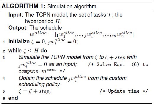
This section describes how to implement a custom schedule. Algorithm 1 provides the executive cycle of the simulator. It includes the scheduler (user defined or pre-programmed one) in line 4.
The main input signals, from the simulation environment, that the user might use,
are the CPU temperature, executed tasks, current CPU frequency and consumed
energy, also the secondary signals
If the user describes the scheduler as a continuous one, then he/she must write the signal walloc as:
If the user describes the scheduler as a discrete one, then he/she must write the
signal
In both cases, the functions represented by the matrices Ai or function ɸ are computed based on the scheduler objectives and task and CPU parameters, as well as the current state of the system. It is the user responsibility the design of such a functions.
Notice that the simulator is time driven, thus, although in the discrete case the
Finally, once the scheduler is defined, it is integrated to the simulation engine and used at each simulation step.
3.5 Building the Global Model
A full system in the simulation framework consists of a set of tasks, a set of CPUs on a platform, and a scheduler (as an input), represented by separated models. In order to simulate a full system, these models must be gathered into a global model. In the case of a continuous scheduler, the global model is simulated by solving the system:
where
4 User Interface
Fig. 6 shows the main window of the simulator GUI. There are three areas, which contain information about Tasks parameters, Processors parameters and Thermal parameters.

The user can manually define the parameters of the tasks set in the area entitled Tasks parameters. The parameters to be defined are the number of tasks, and the value of the WCET, task period and task energy consumption per each task (see Fig. 6a)). Alternatively, a random set of tasks can be configured by checking the UUniFast check box (Fig. 6b)), setting the number of tasks, the utilization of the task set and the interval of periods, and then clicking the button Generate task set.
The area entitled Processors parameters allows to set the number of CPUS and the homogeneous clock frequency. Last, the area Thermal parameters consists of three subareas. The first two correspond to the geometry (length X, height Y, and width Z measurements) and material properties (thermal conductivity k coefficients, density ρ, specific heat capacities Cp ) of the board and CPUs.
The third subarea is for entering the mesh geometry (Mesh step) and the accuracy (dt) of the solutions obtained by the TCPN Thermal model ([17]). Once these parameters have been set, the next step is to select an scheduling policy by clicking the button Select Scheduler in the Scheduler selection tab (Fig. 7). The available scheduling policies appear in a selection list. User-defined scheduling policies will show up in this list too (Fig. 7b)) by following the installation guidelines. A scheduler framework shows the structure of the scheduler for each selected scheduler policy.
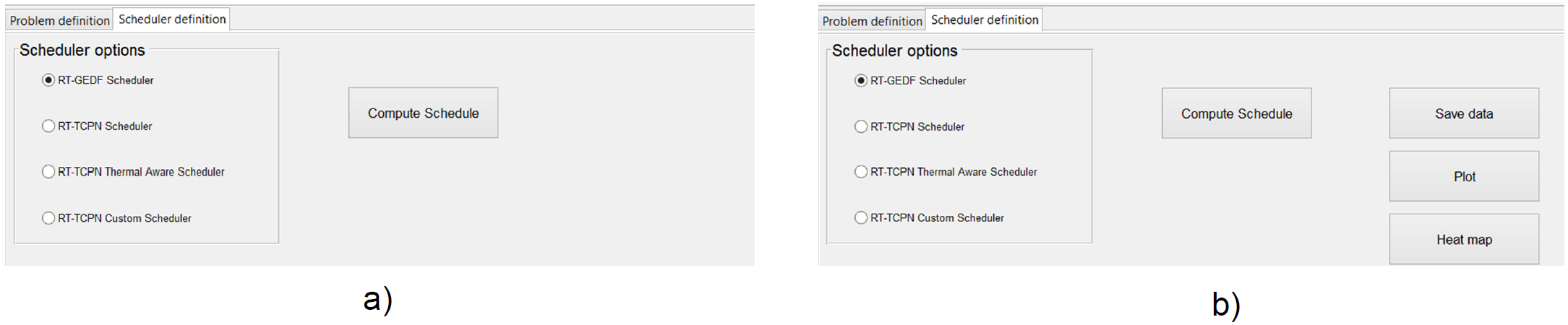
The last step consists in clicking the button Compute Schedule to run the simulation. After a simulation run, the GUI allows to generates plots of the allocation and execution of task's jobs to CPUs and the CPUs temperature evolution. Fig. 7b)) shows the available buttons are: Save data, which save all the simulation data into a file, Plot, which plots task execution and CPU temperature evolution, and Heat map, which is only functional if the user configured the thermal parameters before the simulation.
5 Available Schedulers
This section is intended to show the available schedulers and their implementation in the framework. We only provide global multiprocessor schedulers by the reasons explained in Section 2. The scheduling policies available in the framework are an G-EDF ([1]), an RT fluid scheduler RT-TCPN ([15]), and an RT-TCPNThermal aware scheduler that are describing below.
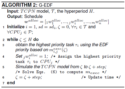
5.1 G-EDF
This scheduler implements a global EDF (G-EDF) algorithm. It is a global
job-level fixed priority scheduling algorithm for sporadic task systems, which
is optimal for implicit-deadline tasks with regard to soft RT constraints
[2].
Jobs are allocated to CPUs from a single queue. The highest priority is assigned
to the job with the earliest absolute deadline. The signal
5.2 RT-TCPN
RT-TCPN is a scheduler based on the TCPN model presented in
[15]. It is composed of a global fluid scheduler
and the discretization of the fluid scheduler. The fluid schedule computation is
limited to every deadline, whereas preemption and context switch occur at every
quantum, at which we check the difference between the actual and the expected
fluid execution. RT-TCPN obtains a discrete schedule that
closely tracks the fluid one (
The algorithm considers the ordered set of all tasks' jobs deadlines to define
scheduling intervals, as in deadline partitioning ([18]). Each task
τi must be executed
where
The actual execution

Fig. 8 depicts the scheme of the algorithm
implemented in this framework. The dotted box A contains a set of signals that
represent the normal behavior of the system. Signal A.1 describes the function

5.3 RT-TCPN Thermal Aware
The schedule computation in this algorithm encompasses temporal and thermal constraints. The temperature of the chip must be kept under a temperature threshold Tmax that depends on system design requirements. The fluid schedule function introduced in [3] is extended to include thermal restrictions. This is achieved by considering the steady state of Eq. 7a, i.e. if the schedule is periodic, fluid and evenly distributed over the hyperperiod, then the temperature must reach a steady state. Thermal Eqs. (7a and 7b) can be rewritten as:
Thus, in a thermal steady state
The steady state temperature
The thermal constraint is derived by combining the last expression and Eq. (17).
The task allocation vector
The first constraint is the thermal constraint. The other two constraints are a
straightforward extension of the time and CPU utilization used in the
RT-TCPN algorithm for the multiprocessor case. The required
fluid schedule function
Considered the sliding surface:
where
Figure 9 shows how the implemented
algorithm works. It is composed of the off-line and online stages. Based on an
LPP, the off-line stage computes the functions

6 Example
We illustrate the usage of the simulation framework with the following experiments. First, we compare the temperature variations of the simulated system as generated by the available schedulers.
In the experiments we assume a platform composed of two homogeneous 1cm × 1cm silicon microprocessors mounted over a 5cm × 5cm copper heat spreader as in [17]. The thickness of the silicon microprocessors and the copper heat spreader are 0.5mm and 1mm respectively.
The experiment considers the task set
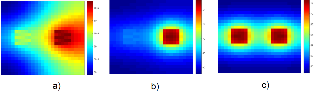
Fig. 10 depicts the temperature obtained by the schedulers for both CPUs. G-EDF and RT-TCPN obtain a feasible schedule, however the resulting temperatures violate the thermal constraint. In contrast, the RT-TCPN Thermal scheduler meets both thermal and temporal requirements. Fig. 11 presents the heat map obtained by the simulator.

7 Conclusion and Future Work
Designing, testing and comparing RT scheduling methods on multiprocessors is a gruesome and time consuming chore, all the more when thermal restrictions are considered. Resorting to a real system implementation is overkilling during the early design stages. We have developed a simulation framework which encompasses modules for defining and modelling tasks, CPUs, thermal properties and three global RT schedulers out-of-the box. It is available at https://www.gdl.cinvestav.mx/art/uploads/ SchedulerFrameworkTCPN.zip and it is distributed as open source software as-is.
The main contribution compared with different real time simulation tools relies on its capability of handling temperature analysis over different scheduling policies, which can be very useful in order to detect thermal management problems that can be solved trough a correction in the scheduling algorithms.
We are working to include a number of improvements such as simpler procedures to replace or customize the thermal, task and CPUs models, additional algorithms to generate task sets and thermal-energy aware schedulers. Following the trend of some current multiprocessors, the framework will also include models for heterogeneous CPUs with per-CPU frequency adjustments.

