


 text new page (beta)
 English (pdf)
 Article in xml format
 Article references
 Send this article by e-mail
 Cited by SciELO
  Similars in
SciELO
Similars in
SciELO 
 Permalink
1 Introduction
Many neurobiologists use the visual system of the fruit fly (Drosophila) as a model to study neuron interaction [4,6,9] and neuron organization into columnar units in the brain and extrapolate this knowledge to human behavior and diseases [5,4,8]. Drosophila studies have a significant value for the scientific community with five Nobel prizes related, because of working and manipulating the genome of the fruit fly is an easily reproducible technique and a big amount of genetic tools are available. Additionally, this animal shows a relatively complex behavioral repertoire in a relatively simply organized brain, with only 100,000 neurons. Within the fly, the optic lobe is especially appealing because flies are highly visual animals, with the two optic lobes encompassing approximately 50% of the total brain volume.
The fluorescence microscopy images of columns commonly have high contrast. However, the detection is compromised by background signals, generating fuzzy boundaries of columns. Additionally, the number of elements are approximately 103 [6]. Therefore, the detection and counting of columns are still difficult due to the manual analysis nature that involves the technique. An automated detection, counting, segmentation and morphologic analysis of columns can provide to researchers a significant advantage on speed and accuracy in the analysis of this kind of images.
The main aim of this work is to develop an algorithm for real-time shape recognition, counting, and classification of the Drosophila pupa visual ganglia column images obtained by using a confocal microscope. The main contribution of this algorithm is that we combine automatic operations with image analysis results and user parameters in real-time.
This paper is divided into four sections. In the next section, we present the methods and data for the image processing algorithm (including its limitations), detection, segmentation, and the decision tree algorithm to obtain the rules which define a set of good shape or bad shape columns. In section 3, we present our images analysis results. Finally, in section 4, we provide conclusions.
2 Data and Methods
In this section we describe the data and propose a real-time semi-automatic image processing algorithm to detect, visualize, find edges, compute the position (centroid) for fluorescence of optic lobule fly pupae images.
2.1 Data
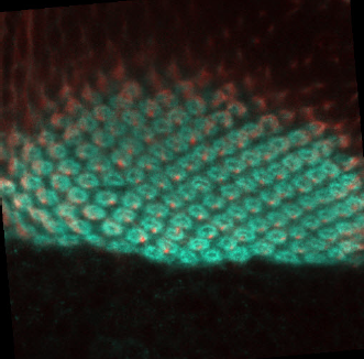
We have used 12 fluorescence microscopy images (120 segmented shapes) which were provided and labeled by the research team of the Laboratory of Developmental Neurobiology of the Kanazawa University in Kanazawa, Ishikawa Prefecture, Japan. They were handed to our team as 8bit-RGB, JPEG images of 500x500 pixels, Figure 1 shows an example of original images.
2.2 Image Processing
We have used Open CV 3.0 [7] with Python to develop our real-time image processing and analysis of a selected Region of Interest (ROI) selected by the user, with a fixed size 150 x 150 pixels.
The algorithm to detect and segment cell-shapes is described as follows:
RGB image is converted into gray 8-bit grayscale.
Bilateral filter is applied to the gray image ROI [3]. This filter is highly effective in noise removal while keeping edges sharp.
An adaptive binary threshold operation is used, with an initial threshold C0 value of -3. However, the user can define the C.
A dilate operation is applied to approximate the real size of the detected shapes.
The contours shapes are obtained from the binary image with the method [10].
Compute the proportion between width and height and compare with the main value of the other shapes.
The centroids are computed to count the possible cells and serves as a visual aid.
Draw the visual shape over the first copy of the squared image (as shown in Fig 4).
The main contribution of this image prepossessing algorithm is that, we can combine automatic image processing with image analysis, and user parameters to fine-tune the results and display them in real-time. It is possible to see and download this code1.
2.3 Image Processing Limitations
Due to the extremely variable quality of the microscopic image, even at same the anatomic region, we measure the range of Signal to Noise Ratio (SNR), where our algorithm is reliable. To measure the SNR we used the mean value of the pixel intensity L as a signal and variance as a noise (of a normal distribution) of some Regions of Interest (ROI) with gray images. The SNR can be obtained as follows:
In the case that the image has a low value of SNR the user has the option to select or remove detected shapes individually as necessary.
2.4 Image Analysis and Feature Extraction
The image analysis computation is focused in two main areas compute the number of possible shapes of the column and obtaining features for their classification. We use the expertise of the laboratory team and our experimental results in order to define the main features. The main features were the width, height, perimeter, area, the centroid of each segmented shape. In addition, the main shape analysis measurements and operations are:
2.5 Cell Classification
We have segmented 120 shape cells and, with the help of the neurobiology laboratory team of the University of Kanazawa, we obtain two labels GOOD and BAD cells.
In order to do the image cell classification, we use the shape as a principal feature. We used a decision tree not only to obtain a prediction or classification result but also to obtain logical rules with a simple explanation. These rules can be correlated with the features of the anatomical shapes, expressed by the experts. It is worth to mention that the decision tree can compute an accurate value, even with little data and it is not a black box algorithm [12].
To create the decision tree we used Weka [11,12]. The JRip algorithm [2] was used to classify the good and bad cells, with 10 folds cross-validation. To create the training input information we propose the following input features:
3 Results
3.1 Image Processing
The real-time image processing steps are presented in Figure 2. The RGB image is converted into 8-bit grayscale, then bilateral filter is applied to the gray image, after that, an adaptive binary threshold operation is used, finally, a dilate operation is applied.
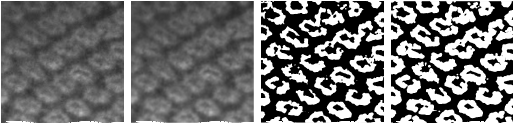
Fig. 2 From left to right: 8 bit gray scale ROI transform, bilateral filter application, adaptive threshold, and dilate operation
The contours shapes from the binary image, we compute the centroids to count the number of cells and draw the visual shape over the first copy of the squared image (See Figure 3)

3.2 Image Processing Limitations
The SNR has been measured for each ROI. According to our measures, the proposed algorithm works better with SNR > 4.7, this value is closer to Rose criteria value [1].
In Figure 4 we show an example of the ROI of an image with SNR = 3.6, in this case, the algorithm has the ability to detect several shapes (white contours), but has some false positive results. Even with this SNR, the user can filter easily in the application the bad shapes and not include them in the count.
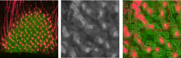
Fig. 4 Original image (left), ROI of image processed ROI image with SNR = 3.67 (center), and result of processing at the ROI (right)
Figure 5 shows the worst quality image that we have in our experiments. In this case the SNR = 2.7, and even in these conditions, our algorithm can detect some regular cell shapes.
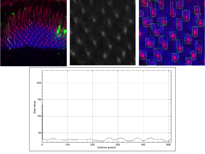
Fig. 5 Worst SNR image (SNR = 2.7) of the set. Original image (left), ROI(center), and the result of the segmentation (left). In the bottom part, we present a plot profile of the ROI
However, the perimeter, area defined by each shape, is highly incorrect. We show the original image, the ROI, and the segmented images. Additionally, in this case, we present a plot profile with the intensity of the pixel L, it is possible to see that there almost the same signal of the cells and the background.
3.3 Image Analysis
In Table 1 we present the mean value and the standard deviation of feateures (F) WHPROPORTION=W/H, PXA, CHANGESX=CHX and CHANGESY=CHY. of both classes (C) good (G) and bad (B). According to the results, the feature mean values and their standard deviation in both classes are crossing. As a consequence, is complicated to use of only a statistical method to define good cells from the bad ones.
Table 1 Image analysis results
| F/C | W/H | PXA | CHX | CHY |
|---|---|---|---|---|
| G | 1.4±0.2 | 32.9±12.2 | 3.3±0.9 | 2.7±0.6 |
| B | 1.5±0.4 | 24.3±7.0 | 4.0±1.1 | 3.6±1.1 |
Additionally, we count the number of cells and each position. We use CENTROID to calculate how many cells are, their position in the image, and their classification. Moreover, we obtain some heuristic rules, that we used to improve the shape detection. The set of heuristic rules are:
Remove very small shapes, most likely created from remaining noise (perimeter < 30 pixels).
Remove the shapes that are totally enclosed by others, this is to avoid toroid-like shapes.
Remove the areas greater than 1.5 standard deviations (also show as a visual aid).
Remove all the incomplete forms and remove the shapes that more than 50% of the area is outside ROI.
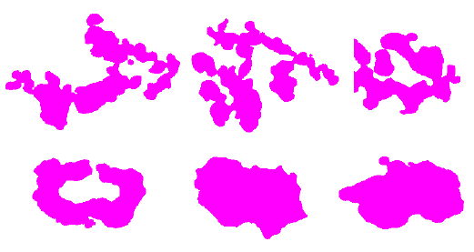
Examples of good and bad shapes are shown in Figure 6. It is easy to see that the good cells are more rounded. In the case of the bad cells, their shape is irregular and speculated.
3.4 Shape Classification
The accuracy of the shape classification of the cells was 75%, with a Kappa statistic of 0.5031. The set of rules created are by the proposed decision-three are:
IF Perimeter and Area (PXA >= 33.42) ISGOOD=1 (53.0/8.0).
IF average changes of color in Y (CHANGESY <= 3.27) and proportion between width and height (WHPROPORTION 1.46 <= 1.63) ISGOOD = 1 (15.0/2.0).
IF (CHANGESY <= 2.51) ISGOOD = 1 (11.0/3.0).
ELSE ISGOOD = 0(92.0/15.0).
The rules obtained are consistent with the expert criteria. However, in future work, we want to explore to a convolutional neural network in order to evaluate the classification of the shapes.
3.5 CC Analyzer GUI
The GUI and the full code is available at https://github.com/enriqueav/CCAnalyzer the Figure 7 where is shown the shape, variables, the count of the cells and the result of the classification. It is possible to see the contour of the enclosing rectangles for each of the detected shape. Rectangles are printed using 2 different colors: green when the shape is marked as good shape and red when the shape is marked as bad shape.

Additionally, the computed cell shape is presented in white and the centroid is drawing in orange. We believe that this GUI can be useful to create a bigger dataset in order to improve the shape classification.
4 Conclusions
We have presented our real-time algorithms to detect, count and classify correct and disorganized columns of the optic lobe of Drosophila pupae. In this paper we present a real-time image processing method for an ROI to detect cell contour-shapes, using the analysis information, we get and heuristic rules to detect the cell shapes. Additionally, we have used the signal to noise ratio of the ROI. We conclude that a (SNR > 4.7) guarantee a 75% (with a Kappa statistic of 0.50) of accuracy or more in the shape classification using our decision tree rules. One of the main contributions of these algorithms is that we combine automatic operations, with image analysis results, machine learning techniques, and user parameters in real-time to obtain a more reliable result.
Finally, we present a desktop application using Python and OpenCV 3.0. The results in the GUI are visible in real-time, giving the user enormous flexibility and ability to choose the desired ROI and apply post-processing operations. We believe that this GUI can be useful to create a bigger dataset in order to improve the shape classification even for other applications.

