


 text new page (beta)
 English (pdf)
 Article in xml format
 Article references
 Send this article by e-mail
 Cited by SciELO
  Similars in
SciELO
Similars in
SciELO 
 Permalink
1 Introduction
Image segmentation is the process of image partition into homogeneous regions (sets or pixels) that share certain visual characteristics [1,2]. The objective of segmentation is to simplify and/or change the representation of an image into something that is more meaningful and easier to analyze [3]. Generally image segmentation depends on threshold dependent criteria [4].Otsu method is a classical technique frequently applied to image segmentation [5]. More recently, in field of image segmentation, researchers have extensively worked over this fundamental problem and applied various algorithms/methods. One of these algorithms is Artificial Neural Networks (ANN)[6]. The interest on ANNs has been on the rise due to them being inspired on the nervous system, their usefulness for solving pattern recognition problems and their parallel architectures [7].
ANN can change their responses according to the environmental conditions and learn from experience [8]. It has been seen that ANN is a good approach to analyze images and segment different objects present in a given image [4]. ANN has been used for image segmentation based on its supervised and unsupervised methods [9].
In the segmentation of color images, unsupervised learning is preferred to supervised learning because the latter requires a set of training samples, which may not always be available [6,10]. The Self-Organizing Maps (SOM), a widely used image segmentation algorithm [2], is a type of unsupervised ANN [11].
The SOM features are very useful in data analysis and data visualization, which makes it an important tool in image segmentation [8]. It has two major characteristics, (i) it produces a low dimensional representation of the input space (ii) it groups together similar samples [9].
These two characteristics of SOM help us in segmenting the regions of the image that has similar features, and it reduces the number of colors required to represent an image [6]. SOM studies each input component and then classifies the input into the corresponding class (color). The basic Self-Organizing Maps (SOM) 18. Neural Network consists of the input layer and the output layer, which is fully connected with the input layer by the adjusted weights (prototype vectors). The number of units in the input layer corresponds to the dimension of the data. The number of units in the output layer is the number of reference vectors in the data space (image).
In SOM, the high-dimensional input vectors are projected in a nonlinear way to a low-dimensional map (usually a two-dimensional space), and SOM can perform this transformation adaptively in a topologically ordered fashion. Therefore, the neurons are placed at the nodes of a two-dimensional lattice.
Every neuron of the map is represented by an n-dimensional weight vector (prototype vector), θ=[ θ_1,…, θ_n], where θ denotes the dimension of the input vectors. The prototype vectors together form a codebook. The units (neurons) of the map are connected to adjacent ones by a neighborhood relation, which indicates the topology of the map. SOM can adjust the weight vectors of adjacent units in the competitive layer by competitive learning.
In the training (learning) phase, the SOM forms an elastic net that folds onto the "cloud" formed by the input data. Similar input vectors should be mapped close together on the nearby neurons, and group them into clusters.
SOM is an unsupervised classification which is used to cluster a data set based on statistics only, and can be trained by an unsupervised learning algorithm in which the network learns to form its own classifications of training data without external help.
The SOM is trained iteratively. Recently, many researchers have explored the alone Self-Organizing Maps (SOM) Neural Network capabilities in image segmentation and proposed several models for object shape recovery [12], to deal with images containing regions characterized by intensity in homogeneity [13] or to segment a Landsat image [14].
In addition, many researchers have explored the SOM capabilities combined with other techniques for brain image segmentation [15] or to identify the water region from LANDSAT satellite image [16]. However, the choice of image segmentation technique depends on the problem being considered [17]. In this paper, a threshold color image segmentation methodology based on SOM Neural Network is presented.
In this paper, a threshold color image segmentation methodology based on SOM Neural Network is presented.
The objective of the segmentation methodology is to identify and separate the seed castor (Ricinus comunnis L) to determine the minimum number of color features.
The remainder of this paper is organized as follows. In Section 2, the images analyzed in our experiments and methodology are presented. In Section 3, we show the experimental results obtained by the proposed methodology. Finally, Section 4 contains the conclusions of this research.
2 Material and Methods
2.1 Material
In this paper, the color image segmentation methodology segments seed castor ricinus images ("nh1", "nh2", "nh3", "nh4", "nh5" y "nh6") and two standard test images ("House" and "Girl").
The seed collections were supplied by the National Research Institute for Forestry, Agriculture and Livestock (in Spanish: Instituto Nacional de Investigaciones Forestales, Agrícolas y Pecuarias, INIFAP) of Mexico at the Bajío.
Standard images were obtained from University of Southern California1 in miscellaneous section.
Seed images were acquired under standard conditions using a microtouch (Dinolite digital microscope) over a white background at 29 cm.
Images were stored in the Joint Photographic Experts Group (JPG) format (480 x 640 pixels color image).
Figure 1 shows a representative set of the six castor lines analyzed. Standard images have a TIFF format with dimensions of 256x256 color image and 96 ppp.

Figure 1a shows the image for nh1, 1b for nh2, 1c for nh3, 1d for nh4, 1e for nh5 and 1f for nh6.
2.2 Methodology
With the objective of determining the minimum number of color features in six seed lines (nh1, nh2, nh3, nh4, nh5 and nh6) of castor (Ricinus comunnis L.) for future seed characterization process, a color image segmentation methodology is presented. Figure 2 illustrates the segmentation methodology.

The segmentation methodology starts setting the maximum number of experiments, the maximum number of SOM number of image segments. Then segmentation process segments the image in an increasing way. If the SOM process finds an empty class, the process selects the previous SOM network and ends. On the other hand, the process increments one neuron and another SOM network is created.
The number of neurons in SOM is increased until one of them is empty. When SOM process finds an empty class, it is considered that selected network represents the minimum number of segments in image. The main steps of the SOM methodology are described in algorithm 1.
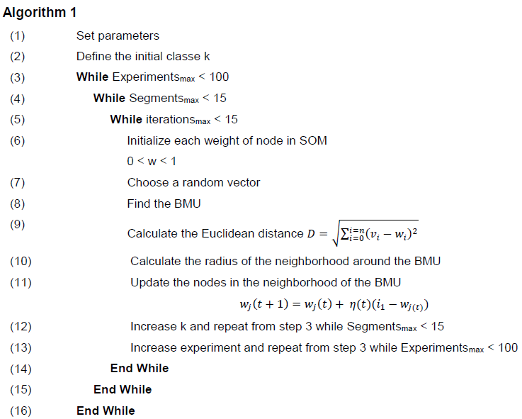
In the first step, segmentation process selects an initial number of k classes. In second step, SOM method segments the image into the k selected classes. If the SOM process found an empty class, the processes end and selects the previous SOM network to represents the segmented image.
On the other hand, the SOM process increments one class and another SOM network is created with an additional neuron to segment the image. The number of neurons in SOM is increased until one of them is empty.
3 Experimental Results
This section presents the obtained results. Six seed lines ("nh1", "nh2", "nh3", "nh4", "nh5" and "nh6") of seed castor (Ricinus comunnis L.) are used for conducting experiments. Two standard test images ("House" and "Girl") obtained from University of Southern California in Miscellaneous section were also used for testing. According to section 2B, table 1 shows the implemented SOM network parameters.
Table 1 SOM network parameters
| Parameters | Values |
|---|---|
| Number of iterations | 100 |
| Number of experiments | 100 |
| Number of segments | 15 |
| Initial segment | 2 |
| input data | $480 x 640 x 3$ |
| SOM network structure | [1 1 3] |
| Distance type | Euclidean |
3.1 Image Segmentation Results
This section shows the results obtained by different network structures for each seed image. Figure 3 shows the image segmentation results by the applied methodology. From top to bottom, they are "nh1", "nh2", "nh3", "nh4", "nh5" and "nh6" seed images and "House" and "Girl" standard images. The first column to the seven columns show, respectively, the corresponding images of segmentation results with two to eight thresholds obtained by the methodology.

For nh1 seed image, the figure with the minimum number of segments is Figure 3(a5), for nh2 is Figure 3(b3), for nh3 is Figure 3(c3), for nh4 is Figure 3(d4), for nh5 is Figure 3(e5), for nh6 is Figure 3(f4).
For house standard image, figure 3(g8) shows the minimum number of segments. In the case of the Girl image, the process not found a minimum number of segments to represent the image. In all process, the experiments were extended to 15 segments. Figures 3(h1) to 3(h7) show the process for eight segments.
For seed images, something important to emphasize is the segmentation of their shadows that allow the measure of their dimensions. However, as we show in the background of figures 3(a6) or 3(b4), with the number of k threshold increasing, some segments of the image are distortional.
3.2 Accuracy Evaluation
A numerical representation of the best results obtained by the methodology are shown in tables II, III, IV, V, VI, VII for the seed lines. For House and Girl standard images, tables VIII and IX show the number of pixels segmented for the threshold values. In all tables, the best segmentation results are emphasized in boldface.
Table 2 Threshold values for nh1
| Image | k | Threshold | |||||||||
|---|---|---|---|---|---|---|---|---|---|---|---|
| 2 | 0.7094, | 0.0107 | |||||||||
| 3 | 0.5073, | 0.0245, | 0.8879 | ||||||||
| 4 | 0.9871, | 0.0302, | 0.6800, | 0.3846 | |||||||
| 5 | 0.0485, | 0.4599, | 0.7178, | 1.0067, | 0.1252 | ||||||
| nh1 | 6 | 0.0558, | 0.0615, | 0.7763, | 0.5769, | 0.3562, | 1.0309 | ||||
| 7 | 0.0615, | 0.5769, | 1.0309, | 0.3562, | 0.3918, | 0.0558, | 0.7763 | ||||
| 8 | 0.0650, | 0.7711, | 0.2774, | 0.4784, | 0.0394, | 0.6562, | 0.8269, | 1.0499 | |||
| 9 | 0.6466, | 0.8655, | 0.0615, | 0.3562, | 0.5769, | 0.6962, | 0.7763, | 0.0558, | 1.0309 | ||
| 10 | 0.5769, | 0.7763, | 0.3562, | 0.6321, | 0.5926, | 0.0615, | 0.7449, | 0.0558, | 1.0309, | 0.6815 |
Table 3 Threshold values for nh2
| Image | k | Threshold | |||||||||
|---|---|---|---|---|---|---|---|---|---|---|---|
| 2 | 0.7448, | 0.0335 | |||||||||
| 3 | 0.5122, | 0.9119, | 0.04517 | ||||||||
| 4 | 0.6520, | 0.9630, | 0.3255, | 0.0517 | |||||||
| 5 | 0.3255, | 0.7013, | 0.9630, | 0.0517, | 0.6520 | ||||||
| nh2 | 6 | 0.4358, | 0.0517, | 0.9630, | 0.3255, | 0.7820, | 0.6520 | ||||
| 7 | 0.6280, | 0.0748, | 0.4157, | 0.9766, | 0.6078, | 0.6916, | 0.062275245 | ||||
| 8 | 0.2162, | 1.0155, | 0.0173, | 0.6388, | 0.4414, | 0.8243, | 0.0861, | 0.7758 | |||
| 9 | 0.5609, | 0.0320, | 0.3165, | 0.5397, | 0.5599, | 0.9988, | 0.0814, | 0.7676, | 0.6882 | ||
| 10 | 0.6439, | 0.8243, | 0.6995, | 0.6388, | 0.0861, | 0.2771, | 0.4414, | 1.0155, | 0.2162, | 0.0173 |
Table 4 Threshold values for nh3
| Image | k | Threshold | |||||||||
|---|---|---|---|---|---|---|---|---|---|---|---|
| 2 | 0.4880, | 0.0282 | |||||||||
| 3 | 0.7061, | 0.0282, | 0.4880 | ||||||||
| 4 | 0.0535, | 0.8358, | 0.2451 | 0.4779 | |||||||
| nh3 | 5 | 0.2451, | 0.6461, | 0.4779, | 0.0535, | 0.8358 | |||||
| 6 | 0.0816, | 0.4042, | 0.2550, | 0.0666, | 0.8955, | 0.6269 | |||||
| 7 | 0.0378, | 0.0745, | 0.9051, | 0.3133, | 0.1916, | 0.4514, | 0.6544 | ||||
| 8 | 0.8955, | 0.2578, | 0.2550, | 0.0666, | 0.6193, | 0.4042, | 0.0816, | 0.6269 | |||
| 9 | 0.8831, | 0.3496, | 0.5751, | 0.1742, | 0.3383, | 0.2214, | 0.4695, | 0.5935, | 0.0585 | ||
| 10 | 0.6269, | 0.7603, | 0.0666, | 0.2550, | 0.0816, | 0.8955, | 0.4042, | 0.4145, | 0.6443, | 0.5123 |
Table 5 Threshold values for nh4
| Image | k | Threshold | |||||||||
|---|---|---|---|---|---|---|---|---|---|---|---|
| 2 | 0.4880 | ||||||||||
| 3 | 0.3085, | 0.0489, | 0.7488 | ||||||||
| 4 | 0.8358, | 0.0535, | 0.2451, | 0.4779 | |||||||
| 5 | 0.8358, | 0.2451, | 0.0535, | 0.7457, | 0.4779 | ||||||
| nh4 | 6 | 0.5935, | 0.0585, | 0.6122, | 0.3496, | 0.8831, | 0.1742 | ||||
| 7 | 0.8003, | 0.4779, | 0.2451, | 0.0535, | 0.7836, | 0.8358, | 0.7471 | ||||
| 8 | 0.0666, | 0.2550, | 0.6164, | 0.8955, | 0.4042, | 0.0816, | 0.6269, | 0.6292 | |||
| 9 | 0.0816, | 0.3702, | 0.2373, | 0.8955, | 0.0666, | 0.2550, | 0.5246, | 0.6269, | 0.4042 | ||
| 10 | 0.2564, | 0.0931, | 0.3911, | 0.5456, | 0.0316, | 0.3814, | 0.1168, | 0.9272, | 0.6386, | 0.7235 |
Table 6 Threshold values for nh5
| Image | k | Threshold | |||||||||
|---|---|---|---|---|---|---|---|---|---|---|---|
| 2 | 0.0139, | 0.6460 | |||||||||
| 3 | 0.0303, | 0.4406, | 0.7890 | ||||||||
| 4 | 0.8998, | 0.6184, | 0.3353, | 0.0358 | |||||||
| 5 | 0.4150, | 0.1156, | 0.0524, | 0.9199, | 0.6546 | ||||||
| nh5 | 6 | 0.9199, | 0.4150, | 0.1156, | 0.6546, | 0.0524, | 0.3140 | ||||
| 7 | 0.6993, | 0.9412, | 0.3079, | 0.3874, | 0.5131, | 0.0621, | 0.0537 | ||||
| 8 | 0.7561, | 0.6022, | 0.0302, | 0.0681, | 0.4355, | 0.9657, | 0.2448, | 0.7089 | |||
| 9 | 0.6470, | 0.3557, | 0.0715, | 0.0167, | 0.9787, | 0.1820, | 0.7907, | 0.5056, | 0.4119 | ||
| 10 | 0.6022, | 0.0681, | 0.9657, | 0.2448, | 0.4355, | 0.3187, | 0.6133, | 0.0302, | 0.2601, | 0.7561 |
Table 7 Threshold values for nh6
| Image | k | Threshold | |||||||||
|---|---|---|---|---|---|---|---|---|---|---|---|
| 2 | 0.0139, | 0.6843 | |||||||||
| 3 | 0.4667, | 0.0369, | 0.8460 | ||||||||
| 4 | 0.0456, | 0.3392, | 0.9411, | 0.6384 | |||||||
| 5 | 0.3392, | 0.9411, | 0.6384, | 0.0456, | 0.5783 | ||||||
| nh6 | 6 | 0.9618, | 0.0643, | 0.4346, | 0.6843, | 0.1285, | 0.2820 | ||||
| 7 | 0.8028, | 1.0090, | 0.2650, | 0.6366, | 0.0389, | 0.4627, | 0.0782 | ||||
| 8 | 0.7395, | 0.7321, | 0.0748, | 0.0570, | 0.3165, | 0.9817, | 0.5323, | 0.7126 | |||
| 9 | 0.8361, | 0.5286, | 0.1972, | 0.3731, | 1.0212, | 0.0820, | 0.6787, | 0.0208, | 0.4602 | ||
| 10 | 0.6366, | 0.0782, | 1.0090, | 0.0389, | 0.4627, | 0.3143, | 0.6641, | 0.2650, | 0.2441, | 0.8028 |
Table 8 Threshold values for house image
| Image | k | Threshold | |||||||||
|---|---|---|---|---|---|---|---|---|---|---|---|
| 2 | 0.3874, | 0.1353 | |||||||||
| 3 | 0.2391, | 0.1449, | 0.5375 | ||||||||
| 4 | 0.5373, | 0.6698, | 0.1449, | 0.2390 | |||||||
| 5 | 0.2256, | 0.6698, | 0.3969, | 0.6142, | 0.1446 | ||||||
| House | 6 | 0.1465, | 0.2955, | 0.6698, | 0.6135, | 0.3953, | 0.2286 | ||||
| 7 | 0.6698, | 0.1464, | 0.6831, | 0.3953, | 0.2286, | 0.2955, | 0.6135 | ||||
| 8 | 0.1519, | 0.3807, | 0.5352, | 0.7102, | 0.6698, | 0.2987, | 0.1968, | 0.2344 | |||
| 9 | 0.2987, | 0.6698, | 0.5352, | 0.2344, | 0.7226, | 0.7102, | 0.1968, | 0.1519, | 0.3807 | ||
| 10 | 0.2352, | 0.5357, | 0.3817, | 0.7105, | 0.2041, | 0.4775, | 0.3134, | 0.6698, | 0.0560, | 0.1560 |
Table 9 Threshold values for girl image
| Image | k | Threshold | |||||||||
|---|---|---|---|---|---|---|---|---|---|---|---|
| 2 | 0.6607, | 0.1493, | |||||||||
| 3 | 0.6517, | 0.8824, | 0.1787, | ||||||||
| 4 | 0.3765, | 0.6689, | 0.9197, | 0.1064 | |||||||
| 5 | 0.3742, | 0.1061, | 0.9535, | 0.6948, | 0.6526 | ||||||
| Girl | 6 | 0.4653, | 0.1110, | 0.6756, | 0.6907, | 0.9750, | 0.2918 | ||||
| 7 | 0.2929, | 0.1103, | 0.6045, | 0.6814, | 0.4655, | 0.9762, | 0.7102 | ||||
| 8 | 0.2914, | 0.5080, | 0.6230, | 0.7242, | 0.9832, | 0.7136, | 0.1104, | 0.4673 | |||
| 9 | 0.3484, | 0.5294, | 0.2988, | 0.7303, | 0.9845, | 0.7193, | 0.6613, | 0.1101, | 0.4719 | ||
| 10 | 0.7200, | 0.3057, | 0.4389, | 0.9848, | 0.1835, | 0.5326, | 0.4761, | 0.7318, | 0.6696, | 0.0673 |
It can be found that for nh1 the algorithm obtain the minimum representation when k=6, for nh2 when k=4, for nh3 when k=4, for nh4 K=5, for nh5 when K=6 and for nh6 when k=5. For standard House image, table VIII shows the minimum representation when k=8. As mentioned previously, in case of the Girl image, the SOM process not found a minimum number of segments to represent the image until 15 segments.
3.3 Stability Evaluation
For stability evaluation, tables X, XI, XII, XIII, XIV and XV show the segmented pixels for each seed line. The best results are emphasized in boldface.
Table 10 Number of pixels for nh1
| Image | k | Pixels | |||||||||
|---|---|---|---|---|---|---|---|---|---|---|---|
| 2 | 110379, | 196821 | |||||||||
| 3 | 66741, | 186472, | 53987 | ||||||||
| 4 | 31517, | 181754, | 52558, | 41371 | |||||||
| 5 | 154248, | 42405, | 46203, | 27939, | 36405 | ||||||
| nh1 | 6 | 61733, | 122073, | 34516, | 36715, | 28638, | 23525 | ||||
| 7 | 122073, | 36715, | 23525, | 28638, | 0, | 61733, | 34516 | ||||
| 8 | 112609, | 0, | 19370, | 29452, | 67752, | 32049, | 25753, | 20215 | |||
| 9 | 0, | 0, | 122073, | 28638, | 36715, | 0, | 34516, | 61733, | 23525 | ||
| 10 | 36715, | 34516, | 28638, | 0, | 0, | 122073, | 0, | 61733, | 23525, | 0 |
Table 11 Number of pixels for nh2
| Image | k | Pixels | |||||||||
|---|---|---|---|---|---|---|---|---|---|---|---|
| 2 | 92446, | 214754 | |||||||||
| 3 | 52716, | 48633, | 205851 | ||||||||
| 4 | 42199, | 36775, | 28987, | 199239 | |||||||
| 5 | 28987, | 0, | 36775, | 199239, | 42199 | ||||||
| nh3 | 6 | 0, | 199239, | 36775, | 28987, | 0, | 42199 | ||||
| 7 | 0, | 149567, | 29761, | 33816, | 0, | 37512, | 56544 | ||||
| 8 | 15026, | 24621, | 80228, | 26821, | 21833, | 21589, | 117082, | 0 | |||
| 9 | 29018, | 71738, | 20754, | 0, | 0, | 28633, | 130041, | 27016, | 0 | ||
| 10 | 0, | 21589, | 0, | 26821, | 117082, | 0, | 21833, | 24621, | 15026, | 80228 |
Table 12 Number of pixels for nh3
| Image | k | Pixels | |||||||||
|---|---|---|---|---|---|---|---|---|---|---|---|
| 2 | 92202, | 214998 | |||||||||
| 3 | 0, | 214998, | 92202 | ||||||||
| 4 | 183744, | 20857, | 68696, | 33903 | |||||||
| 5 | 68696, | 0, | 33903, | 183744, | 20857 | ||||||
| nh4 | 6 | 45898, | 30645, | 48015, | 150529, | 14643, | 17470 | ||||
| 7 | 60430, | 125333, | 13610, | 36943, | 34467, | 21128, | 15289 | ||||
| 8 | 14643, | 0, | 48015, | 150529, | 0, | 30645, | 45898, | 17470 | |||
| 9 | 15901, | 47748, | 0, | 48821, | 0, | 0, | 0, | 20317, | 174413 | ||
| 10 | 17470, | 0, | 150529, | 48015, | 45898, | 14643, | 30645, | 0, | 0, | 0 |
Table 13 Number of pixels for nh4
| Image | k | Pixels | |||||||||
|---|---|---|---|---|---|---|---|---|---|---|---|
| 2 | 92202, | 214998 | |||||||||
| 3 | 86138, | 190111, | 30951 | ||||||||
| 4 | 20857, | 183744, | 68696, | 33903 | |||||||
| 5 | 20857, | 68696, | 183744, | 0, | 33903 | ||||||
| nh4 | 6 | 20317, | 174413, | 0, | 47748, | 15901, | 48821 | ||||
| 7 | 0, | 33903, | 68696, | 183744, | 0, | 20857, | 0 | ||||
| 8 | 150529, | 48015, | 0, | 14643, | 30645, | 45898, | 17470, | 0 | |||
| 9 | 45898, | 0, | 0, | 14643, | 150529, | 48015, | 0, | 17470, | 30645 | ||
| 10 | 40945, | 76719, | 0, | 14631, | 93790, | 28612, | 30031, | 11300, | 0, | 11172 |
Table 14 Number of pixels for nh5
| Image | k | Pixels | |||||||||
|---|---|---|---|---|---|---|---|---|---|---|---|
| 2 | 194533, | 112667 | |||||||||
| 3 | 182467, | 61433, | 63300 | ||||||||
| 4 | 34477, | 54508, | 40916, | 177299 | |||||||
| 5 | 39811, | 38828, | 149676, | 30357, | 48528 | ||||||
| nh5 | 6 | 30357, | 39811, | 38828, | 48528, | 149676, | 0 | ||||
| 7 | 39248, | 25968, | 27228, | 0, | 34573, | 127122, | 53061 | ||||
| 8 | 28106, | 32354, | 63442, | 112677, | 27925, | 21281, | 21415, | 0 | |||
| 9 | 29829, | 21627, | 104333, | 66858, | 18806, | 17685, | 22571, | 25491, | 0 | ||
| 10 | 32354, | 112677, | 21281, | 21415, | 27925, | 0, | 0, | 63442, | 0, | 28106 |
Table 15 Number of pixels for nh6
| Image | k | Pixels | |||||||||
|---|---|---|---|---|---|---|---|---|---|---|---|
| 2 | 192089, | 115111 | |||||||||
| 3 | 68612, | 179389, | 59199 | ||||||||
| 4 | 173430, | 41514, | 33298, | 58958 | |||||||
| 5 | 41514, | 33298, | 58958, | 173430, | 0 | ||||||
| nh6 | 6 | 28729, | 151350, | 42334, | 50448, | 34339, | 0 | ||||
| 7 | 25948, | 19641, | 21849, | 35358, | 51665, | 30488, | 122251 | ||||
| 8 | 0, | 39925, | 130406, | 46485, | 27527, | 24677, | 38180, | 0 | |||
| 9 | 21098, | 28197, | 16239, | 22428, | 17430, | 112211, | 31975, | 57622, | 0 | ||
| 10 | 35358, | 122251, | 19641, | 51665, | 30488, | 0, | 0, | 21849, | 0, | 25948 |
For nh1, due to in the K=7 segmentation result the algorithm obtain an empty neuron, the methodology select the value of k=6. This value is also obtained when k=9 and K=10. For nh2, the selected value was K=4. This value is also obtained when K=6. For nh3 the selected value was K=4. For nh4 was K=4, this value is also obtained when K=6. For nh5 was K=5 and for nh6 was K=4. Tables XVI and XVII show the segmented pixels for standard images.
Table 16 Number of pixels for house image
| Image | k | Pixels | |||||||||
|---|---|---|---|---|---|---|---|---|---|---|---|
| 2 | 38913, | 26623 | |||||||||
| 3 | 24342, | 25596, | 15598 | ||||||||
| 4 | 15361, | 256, | 25596, | 24323 | |||||||
| 5 | 20830, | 256, | 10032, | 8740, | 25678 | ||||||
| House | 6 | 23417, | 2490, | 256, | 8750, | 10073, | 20550 | ||||
| 7 | 256, | 23414, | 3, | 10073, | 20550, | 2490, | 8750 | ||||
| 8 | 21858, | 7201, | 7733, | 3136, | 256, | 2435, | 3097, | 19820 | |||
| 9 | 2435, | 256, | 7733, | 19820, | 0, | 3136, | 3097, | 21858, | 7201 | ||
| 10 | 19765, | 7708, | 7195, | 3124, | 3009, | 6, | 2188, | 256, | 1166, | 21119 |
Table 17 Number of pixels for girl image
| Image | k | Pixels | |||||||||
|---|---|---|---|---|---|---|---|---|---|---|---|
| 2 | 22850, | 42686 | |||||||||
| 3 | 12314, | 6594, | 46628 | ||||||||
| 4 | 25917, | 11401, | 4679, | 23539 | |||||||
| 5 | 25588, | 23395, | 3580, | 6300, | 6673 | ||||||
| Girl | 6 | 10147, | 22813, | 9199, | 3949, | 3171, | 16257 | ||||
| 7 | 16102, | 22648, | 4096, | 3717, | 9966, | 3145, | 5862 | ||||
| 8 | 15782, | 2167, | 4050, | 2923, | 3006, | 5446, | 22674, | 9488 | |||
| 9 | 1919, | 2115, | 15824, | 2758, | 2962, | 4467, | 4386, | 22209, | 8896 | ||
| 10 | 4334, | 16099, | 1778, | 2958, | 7597, | 2088, | 8424, | 2732, | 4146, | 15380 |
3.4 Convergence Evaluation
In order to evaluate the convergence of the obtained results, figure 4 and table XVIII show a summary of the number of pixels that bellow to each threshold in 100 experiments.

Table 18 Average of segmented in 100 times that the algorithm ran
| Classes k |
Seed images | Standard images | ||||||
|---|---|---|---|---|---|---|---|---|
| nh1 | nh2 | nh3 | nh4 | nh5 | nh6 | house | girl | |
| 2 | 2 | 2 | 2 | 2 | 2 | 2 | 2 | 2 |
| 3 | 3 | 3 | 3 | 3 | 3 | 3 | 3 | 3 |
| 4 | 4 | 4 | 4 | 4 | 4 | 3 | 4 | 4 |
| 5 | 5 | 4 | 5 | 4 | 5 | 4 | 5 | 5 |
| 6 | 6 | 5 | 5 | 5 | 5 | 5 | 6 | 6 |
| 7 | 6 | 6 | 6 | 6 | 5 | 4 | 7 | 7 |
| 8 | 7 | 6 | 6 | 6 | 6 | 6 | 8 | 8 |
| 9 | 8 | 7 | 6 | 7 | 6 | 7 | 8 | 9 |
| 10 | 8 | 7 | 7 | 6 | 7 | 7 | 9 | 10 |
3.5 Computational Time Evaluation
Tables XIX and XX show the computational elapsed and the standard deviation obtained in the 100 times. However, it is necessary to calculate the mean value μ and standard deviation std to show the stability.
Table 19 Mean computational time
| Classes k |
Seed images | Standard images | ||||||
|---|---|---|---|---|---|---|---|---|
| nh1 | nh2 | nh3 | nh4 | nh5 | nh6 | house | girl | |
| 2 | 113.7242 | 114.772 | 140.3726 | 145.9877 | 188.16861 | 185.8431 | 42.8439 | 40.628 |
| 3 | 116.7574 | 117.8129 | 140.8579 | 145.8736 | 190.5456 | 188.5461 | 43.4832 | 41.1045 |
| 4 | 119.1461 | 120.152 | 141.9788 | 147.4625 | 193.7347 | 190.681 | 43.6677 | 41.489 |
| 5 | 121.19 | 122.2104 | 143.6273 | 148.7781 | 196.6336 | 193.1109 | 44.3868 | 42.0343 |
| 6 | 123.2374 | 124.1324 | 145.1459 | 150.4769 | 198.7607 | 194.8986 | 44.6526 | 42.4431 |
| 7 | 125.1423 | 126.2949 | 148.33 | 152.4804 | 201.3035 | 197.3598 | 45.2181 | 42.965 |
| 8 | 127.1337 | 128.317 | 148.6636 | 154.1318 | 203.5051 | 199.7161 | 45.705 | 43.4335 |
| 9 | 129.2232 | 130.2506 | 150.0953 | 155.2709 | 204.9444 | 201.814 | 46.2501 | 43.9008 |
| 10 | 131.1884 | 132.1837 | 151.3128 | 156.9613 | 206.9461 | 204.4079 | 46.5627 | 44.37 |
Table 20 Standard deviation
| Classes k |
Seed images | Standard images | ||||||
|---|---|---|---|---|---|---|---|---|
| nh1 | nh2 | nh3 | nh4 | nh5 | nh6 | house | girl | |
| 2 | 0.896 | 0.4084 | 6.8002 | 4.9806 | 4.4234 | 3.8527 | 1.8314 | 0.745 |
| 3 | 1.0676 | 0.796 | 1.788 | 2.3848 | 3.6912 | 3.6427 | 1.9452 | 0.7385 |
| 4 | 1.0749 | 0.84 | 1.7173 | 2.4315 | 3.6417 | 3.8458 | 1.7145 | 0.7796 |
| 5 | 1.0945 | 0.8289 | 1.706 | 2.514 | 4.5955 | 3.3241 | 1.9423 | 0.7931 |
| 6 | 1.0218 | 0.8095 | 1.7175 | 2.6821 | 4.5862 | 3.4614 | 1.8394 | 0.7851 |
| 7 | 1.0548 | 0.8956 | 2.0696 | 2.3397 | 4.8879 | 3.5614 | 1.9652 | 0.7659 |
| 8 | 1.0497 | 0.8323 | 1.2983 | 2.5473 | 6.0568 | 3.8525 | 1.9262 | 0.7947 |
| 9 | 1.0197 | 0.8196 | 1.5655 | 2.609 | 5.1599 | 4.6414 | 1.7972 | 0.8162 |
| 10 | 1.3205 | 0.7588 | 1.5776 | 2.9448 | 4.4379 | 4.3454 | 1.792 | 0.7431 |
The mean value and standard deviation are defined as:
where ne is the number of times the algorithm ran and CC is the value of the computational cost each time.
The mean computational time and standard deviations are obtained in one hundred experiments.
4 Conclusions
This paper presents a color image segmentation methodology based on Self-Organizing Maps (SOM) Neural Network.
It is allowed to segment appropriately the seed pigmentation classes in a single class and to determine the minimum number of color features in six seed lines.
Something important to distinguish in the segmentation process were the seed shadows detected perfectly.
Proposed methodology, segments seed castor ricinus images ("nh1", "nh2", "nh3", "nh4", "nh5" y "nh6") and two standard test images. The seed images were supplied by the National Research Institute for Forestry, Agriculture and Livestock (in Spanish: Instituto Nacional de Investigaciones Forestales, Agrícolas y Pecuarias, INIFAP) of Mexico at the Bajío. We Standard images were conclude that the proposed methodology is a good option because it obtained from University of Southern California. Results were presented both visual and numerical way.

