


 nueva página del texto (beta)
 Inglés (pdf)
 Artículo en XML
 Referencias del artículo
 Enviar artículo por email
 Citado por SciELO
  Similares en
SciELO
Similares en
SciELO 
 Permalink
1 Introduction
The main objective of machine tools is to generate the required machined surfaces. These machine tools work by the application of relative movements between the tool and the workpiece. A cutting edge of the tool removes from the workpiece an amount of material called chip. Machine tools present displacements and/or rotation in their components and some of their degrees of freedom are used in each machine. In general, there are two types of basic movements for the process of chip generation: the main movement and the feed movement. The lathe is a machine tool, and its main characteristic is that the workpiece rotates in the spindle (main movement) and the cutting tool is semi-fixed in the tool holder (feed movement) of the main carriage.
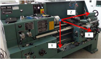
A system of machine tools axes recommend by the International Organization for Standards (ISO) is used, the Z axis of movement is parallel to the axis of rotation of the machine (parallel to the spindle, which provides the main movement of rotation), and the X axis is radial and parallel to the cross slide, the positive displacement in Y is selected in such a way to complete the coordinate system of axes agree with the right-hand rule, in Figure 1 the coordinate axes system for the lathe used in the present paper is shown.
Two-dimensional cutting process (orthogonal cutting) presents of two main orthogonal forces: the cutting force (Fc) and the thrust force (Ft). The first one acts in the direction of the cutting speed and the second one acts in a normal direction to the cutting speed. In figure 2(a) both forces are shown.
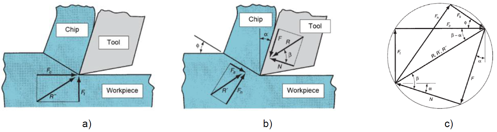
Fig. 2 (a) Orthogonal forces, (b) Friction force and normal force in orthogonal cutting, (c) geometric relationship between forces [1]
Due to the slip between the tool and the workpiece, a friction force (F) acts in a plane parallel to the face of the tool, and the force normal to the friction force (N) acts in a direction perpendicular to the latter, these are shown in figure 2(b).
In figure 2(c), geometric relationship between forces and friction is shown, forces from figure 2(a) and 2(b) are equivalent in 2(c) system.
It is important to estimate the forces that take place in the cutting process and the energy required for the correct design of machine tools to avoid deformations or even failures in its components. Cutting forces and required power are main parameters for a proper selection of a machine tool, because the machine size has a direct impact on initial budget and consumption of energy during its life cycle.
Material removal in any manufacturing process involving chip formation depends on many factors, such as the properties of the raw material, the tool material and the contact conditions between the tool and the workpiece (cutting speed, feed, rake angles, clearance angles, and so on) [2], those characteristics have been experimentally determined for certain types of materials and specific cutting conditions. However, because the development in new materials, it is hard to perform all the experiments for any kind of materials to determine the best parameters and cutting conditions.
Developing a parametric model in which the properties of the involved materials and cutting parameters can be modified, gives the advantage that turning properties can be estimated. When a model can predict the behavior of an unknown process without the necessity of physical experiments, being a virtual model (software simulation) the cost is lower than that of carrying out the experiments on an appropriately equipped machine tool.
2 Background
Ernst and Merchant [3] presented one of the earliest analysis on the topic of orthogonal metal cutting, under the name of "Shear angle solution"; they proposed that the chip behaves as a rigid body, which is maintained in equilibrium by the action of the forces transmitted through the contact zone between the chip and the tool and through the shear plane.
This theory assumes that the angle of the cutting plane (φ) takes a value that minimize the necessary work to perform cutting, the work required for such situation is proportional to the cutting force (Fc). However, this theory is not close to experimental results [3].
The formulation based in obtaining cutting forces in function of the geometric characteristics of the tool and the workpiece, this is, forces in other directions, can be derived.
Lee and Shaffer [3] applied the plasticity theory to the problem of orthogonal metal cutting considering that:
(1) the workpiece material is rigid plastic, this mean that elastic strain are negligible in the deformation process, and once the yield point of the material is reached, the deformation takes place in a constant stress (there is no hardening of the material);
(2) the behavior of the material is independent of the strain per unit of time;
(3) the effects caused by the increase in temperature in the workpiece are neglected; and
(4) the effects of inertia resulting from the acceleration of the material during deformation are neglected.
These assumptions approximate the results obtained to the behavior in plasticity of some of the metallic materials because of the high values for the strain and strains per unit of time during the process. It is known that the hardening per unit of time of some metals decreases rapidly with an increase in strain, and that the effect of a high value of strain per unit of time increase the yield strength of the metal with respect to its ultimate strength. In addition, when there are large strains, the elastic strain is minimal, and tends to be negligible to the total strain. Again, this theory is not close to some experimental results.
Davim and Maranhao [4] studied the cutting process at speeds between 300 m/min and 3000 m/min, in the work developed, they could predict with good precision plastic strain and plastic strain rates.
In their work, it was used a FEA software called ADVANTAGE, the Johnson-Cook model was used as material model and a Coulomb model for friction between the tool and the workpiece. They developed a finite element model capable to predict accurately plastic strain and plastic strain rate with an error of 2.5% and 1.4% respectively in conventional machining (300 m/min), in contrast, whit high machining speeds (3000 m/min), an error of 1.6% and 6.5% respectively was obtained.
Zouhar and Piska [5] used ANSYS LS-DYNA software to represent orthogonal cutting, using the Johnson-Cook formulation as a material failure model for AISI-1045 steel. ANSYS 11 was used, with SOLID element 164. The cutting tool has several geometries and the authors obtain forces, stresses, temperatures and the chip formation.
Martinez et al [6] carried out thermo-mechanical studies, based on finite element, to simulate the orthogonal cutting on AISI-1045 steel parts, considering only the formation of continuous chips. They used DEFORM-2D software and different constitutive models available (Johnson-Cook, Zerilli-Armstrong, Maekawa and Oxley). The authors used constitutive models to simulate the steel behavior and a comparison of the results was made, although the predictions are sensitive to the model used, they concluded that none of the four models is better in all cutting parameters.
In the work of Bil et al [7], several simulation models are compared for the orthogonal cutting process and three different finite element software were used: MSC.Marc, DEFORM-2D, and ADVANTAGE; each software used different friction models and data extrapolation schemes.
They established a threshold for tool penetration as 2 times the contact tolerance value, which in turn is 0.05 times the minimum element length (using a penetration value of 0.0001 mm and 0.0005 mm with an element length of 0.01 mm).
The authors conclude: (1) friction parameter affects the simulation results drastically, but tuning this parameter yields to good concordance only for some variables in the range; (2) a small friction parameter leads to good results for cutting force, whereas other variables (such as thrust force and shear angle) are computed more accurately with large friction parameters; (3) the plain Coulomb friction model is not appropriate for machining purposes since it supplies friction stresses which are larger than the shear yield strength of the material at the tool-chip interface; (4) plain damage models for chip separation are not appropriate for machining purposes, although the remeshing models gives better results; (5) in a typical metal cutting process, very high strain rates are achieved, however, the typical available material data are valid up to strain rates of 40 1/s.
3 Experimental Tests in Lathe
For turning tests, the 3D cutting process is simplified to an orthogonal model, which would be well defined as a two-dimensional model, with depth (or with thickness in the workpiece and in the tool), in other words, it is a three-dimensional model, but where only two-dimensional forces interact in a plane.
To assure orthogonal tests, instead of some full bar, a hollow steel bar is used to avoid any value of thrust force, because this force would demand a three-force analysis.
3.1 Relation between 3D and Orthogonal Cutting
Figure 3 shows several similarities between cutting a hollow bar and orthogonal cutting: the tangential velocity (V) in the outer diameter of the workpiece in the 3D cutting process corresponds to the linear cutting speed (V) in the orthogonal cutting, figure 3(a) and 3(b) respectively.
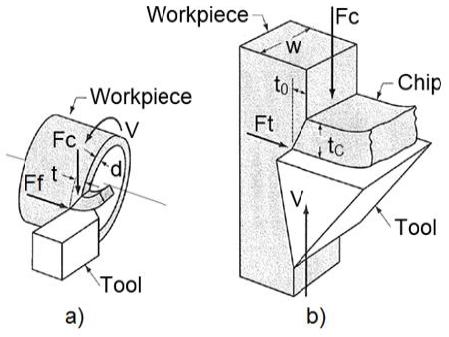
Tool feed movement (f) shown in the 3D model in Figure 3(a) can be represented as the cut depth (t0) in the orthogonal model in Figure 3(b), the cutting depth (d) in 3D turning corresponds to the thickness (w) of the workpiece in the orthogonal model. In the same way with the forces shown, the cutting force (Fc) is the same in both models and the feed force (Ff) in the 3D model corresponds to the thrust force (Ft) in the orthogonal model.
3.2 Orthogonal Cutting Parameters
Previously was stated that tests were performed on a hollow steel bar, which began as a 25.4 mm (1 in) diameter solid bar. The first step was a 22.225 mm (7/8 in) drill to have a 1.5875 mm wall thickness in the hollow bar. The physical measurements shown that the real thickness was 1.6 mm.
According to machining handbooks, for AISI-1045 steel, cutting speeds and feeds for turning are shown in the table 1.
Table 1 Turning speed and feed for AISI-1045 steel [8]
| Speed [ft/min] | Feed [0.001 in/rev] | Feed [mm/rev] |
|---|---|---|
| 00 | 36 | 0.9144 |
| 400 | 17 | 0.4318 |
| 615 | 17 | 0.4318 |
| 815 | 8 | 0.2032 |
A tangential speed of 82.5 ft/min (0.4195 m/s) and a 0.006 in/rev (0.1524 mm/rev) feed was chosen. These conditions correspond to 315 rpm in the spindle, this configuration is provided by SN-32 TRENS lathe.
Rotational spindle speed is obtained with equation 1 [8]:
Different KOMET UNISIX W01-WOHX carbide inserts were used, with different rake angle, table 2 shows the parameters used in orthogonal tests.
3.3 Inserts and Dynamometer
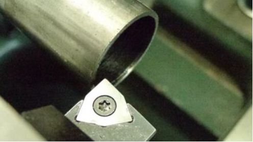
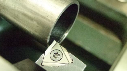
Experimental tests were performed over a pipe mounted in a SN-32 TRENS universal lathe and the force measurement carried out with a TeLC DKM2000 dynamometer with specific holder for KOMET inserts. Figure 4 shows the bar on the chuck in the spindle and the insert 1 in the dynamometer holder to show the force directions used in experimental tests.
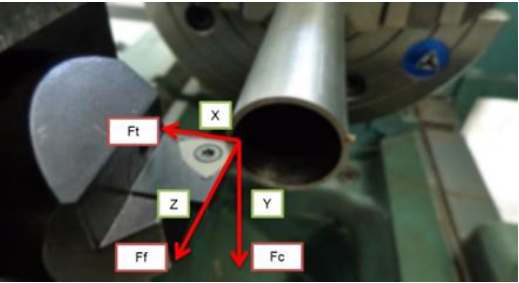
Forces in figure 4 correspond to those described in figure 3(a).
The cutting force and feed force were measured according to the dynamometer design and the figure 3(a) description.
It is expected that thrust force Ft in X direction will be negligible, because the angle of the cutter edge is 90° with the axis spindle, for which this component will not be analyzed (even if experimentally it exists in sometimes although with small values).
Forces in Y and Z directions (cutting force Fc and feed force Ff respectively) are indeed considered.
3.4 Experimental Tests Description
Tests consists in the machining of a hollow bar with 25.4 mm external diameter and a 1.6 mm wall thickness with three different inserts. All of them at the same speeds and feeds. It was established a 315 rpm spindle speed, 0.1524 mm/rev for feed, and tangential speed of 0.4191 m/s (4.2 m/s).
Tests were performed in the following order:

Five experiments were performed per insert type using a new cutting edge in each test.
3.5 Experimental Results
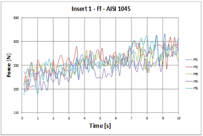
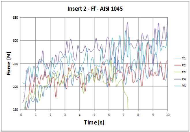
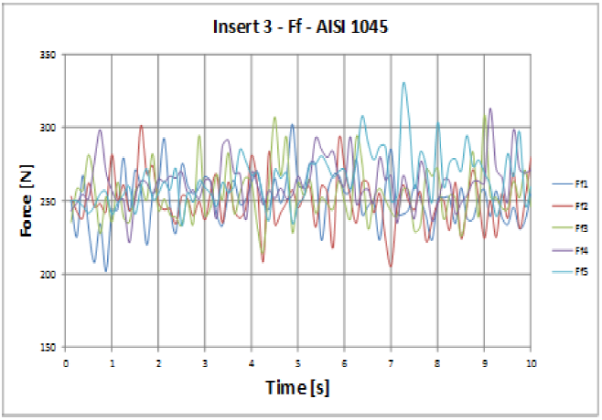
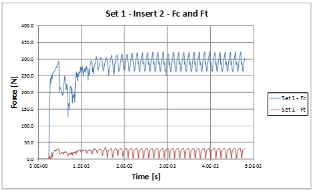
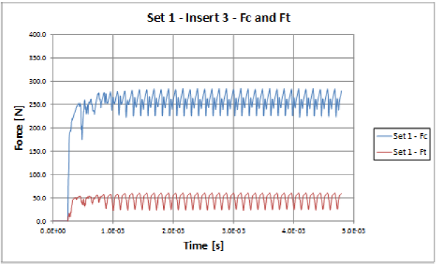
In figures 8-13 measured forces were plot, time is in the abscissa, recorded eight samples per second, since this is the capacity of this dynamometer For cutting force and feed force, initial data was discarded (when insert impacts the material), and plots show the interval that corresponds to the continuous cutting process.
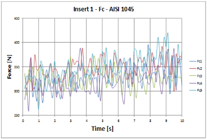
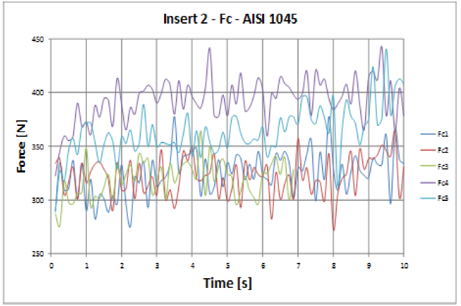
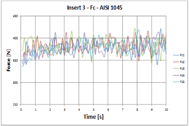
Cutting force is shown in figures 8-10 for inserts 1-3 respectively, the cutting force scale is 250-500 N in the vertical axis.
In figures 11-13 feed force is shown for inserts 1-3 with difference in the scale of the vertical axis 150-350 N versus 250-500 N of cutting force figures.
From graphics, an average value can be obtained for continuous cutting process. Table 3 shows the average forces for the three inserts.
Table 3 Average forces for orthogonal experimental tests
| Force | Insert 1 | Insert 2 | Insert 3 |
|---|---|---|---|
| Cutting force [N] | 337.83 | 345.00 | 381.60 |
| Feed force [N] | 255.35 | 237.28 | 257.42 |
Using the average values, it can be obtained a global friction coefficient for each insert, that considers imperfections presents in the material, angles of tool and workpiece, speeds and feeds, and of course, the real friction between tool and material. Equation 2 establish the relation between tool geometry and forces [4]:
where γ is the clearance angle, and μ is the friction coefficient.
Using equation 2 results in three different friction coefficients for each insert: 0.7559 for insert 1, 0.8547 for insert 2, 1.0356 for insert 3. An average experimental value of 0.8820 is computed from the three last values and literature report a 0.85 friction coefficient for general steels.
4 Simulation by FEM
From comparison between 3D cutting and orthogonal cutting (section 3.1) it can be concluded that feed movement in 3D cutting is the depth of cut in orthogonal model.
In the simulation of the cutting process, cutting depth is set constant (only one revolution was cut without feed movement), and for this reason it is expected that simulated thrust force will be lower than the experimental corresponding, because in simulated cutting doesn't exists carriage movement. Thrust force is generated by the chip through the rake angle. For this reason, only cutting force will be compared.
4.1 Deformable Workpiece
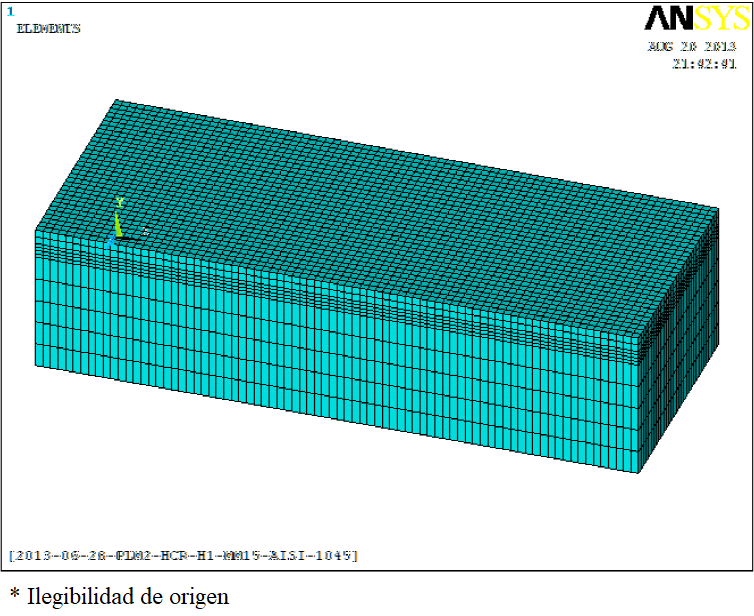
A case of study is proposed where workpiece is represented by a rectangular prismatic geometry, with small dimensions: 4.0 mm in length (X direction), 1.0 mm height (Y direction), and 1.6 mm wide (Z direction). This coordinate axis system corresponds to the used in ANSYS/LSDYNA. It is used a Lagrangian formulation with SOLID 164 element type. Mesh consists in 28160 elements with the follow sizes: 0.10 mm in X direction, 0.05 mm in Z direction, and Y direction has three sizes, 0.16 mm in the bottom, 0.025 mm in the middle, and 0.05 mm in the upper region. Figure 14 shows the meshed workpiece geometry.
It is considered a deformable behavior for the workpiece, Johnson-Cook material model is used and Von Mises stress state equation model for yield stress calculation. Equation 3 [4] shows the stress yield criteria:
Where A is the yield stress, B is the hardening
coefficient,
Material failure occurs when a strain value is achieved, equation 4 shows the failure criteria [4]:
Where D
1
-D
5
are the failure parameters, p is the pressure stress,
and
The simulation of the process test consists in impact of the fixed at the bottom deformable workpiece (set as target) with the insert (set as contact).
It is expected that high stresses will be present during contact, when elements
contacts material and the compression begins. Once a certain strain value
defined by
Table 4 Material properties for AISI-1045 [4 ]
| Parameter | AISI-1045 |
|---|---|
| Density | 7850 kg/m3 |
| Elasticity modulus | 205 GPa |
| Poisson modulus | 0.290 |
| A | 553.1 MPa |
| B | 600.8 MPa |
| C | 0.0134 |
| N | 0.2340 |
| M | 1.0000 |
| 𝑝 | -1e12 |
| D1 | 0.2500 |
| D2 | 4.3800 |
| D3 | 2.6800 |
| D4 | 0.0020 |
| D5 | 0.6100 |
4.2 Tools
To reduce simulation time, it is recommended to simulate only the contact part of the insert geometry, and the most important part is the edge. Figure 15 shows the three inserts, draws were made in CATIA V5 and in figure 16 are shown the geometries used in the simulations Rigid body behavior is selected for inserts, with a linear is isotropic material model. Properties are available in table 5.
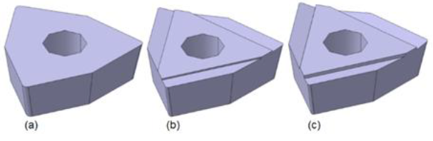
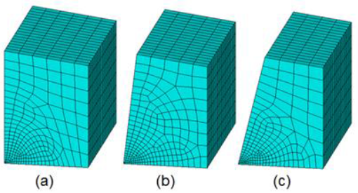
Table 5 Inserts material properties [4]
| Parameter | Carbide inserts |
|---|---|
| Density | 14900 kg/m3 |
| Elasticity modulus | 615 GPa |
| Poisson modulus | 0.220 |
4.3 FEM Simulation Setup
Contact between workpiece and inserts was simulated using an ERODING surface-surface contact type (target and contact part are defined), deformable body is restricted in all its degrees of freedom at the bottom and rigid body can only translate in X direction.
Two sets of simulations were performed, first set with approximate values for solution time, initial speed and the common friction coefficient.
Second set, with calculated parameters for solution time, initial speed and particular friction coefficient. Table 6 resumes the simulation setup for set 1 and set 2.
Table 6 Simulation setup for set 1
| Parameter | Set 1 | Set 2 |
|---|---|---|
| Speed [m/s] | 0.42 | 0.4191 |
| Simulation time [s] | 0.004800 | 0.004772 |
| Friction coefficient | 0.85 | Particular |
Solution was run on Intel core i7-3770 CPU, Windows operative system in 64 bits platform, 16 GB DDR3 1600 MHz RAM and 7200 rpm hard disk drive, each simulation was performed in approximately 27 hours.
4.4 FEM Simulation Set 1
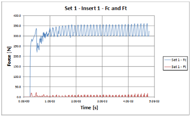
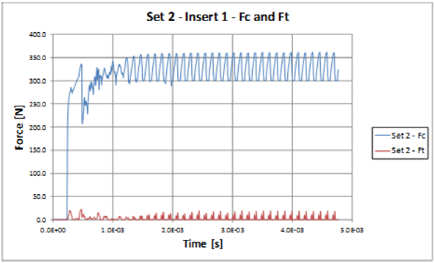
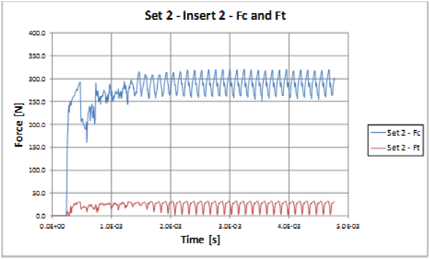
Figures 17-19 shows cutting and thrust force for set 1, with the common friction coefficient. Table 7 shows the average values for the simulated cutting forces (set 1) taken from the steady state of the test (0.0015 s - 0.0045 s).
4.5 FEM Simulation Set 2
Figures 20-22 shows cutting and thrust force for set 2, with friction coefficients: 0.7559, 0.8547, and 0.9999 for insert 1, 2, and 3.
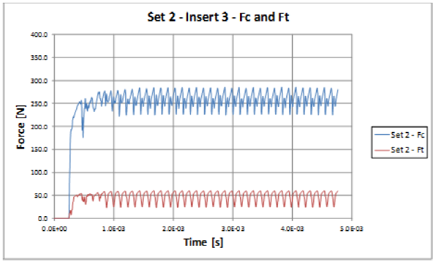
The third friction coefficient was modified because the software only accepts values less than 1.0.
Table 8 shows the average values for the simulated cutting forces (set 2) taken from the steady state of the test (0.0015 s - 0.0045 s).
4.6 Comparative between Simulations and Experimental Results
Once the simulations were performed, the next step is the comparison between both simulations set 1 and set 2 (in set 1 friction coefficient is 0.85 and 0.42 m/s of tangential speed, and set 2 use the experimental friction coefficient for each insert and in all the tangential speed is 0.4191).
Table 9 shows results from set 1 and set 2. It can be observed that modify tangential speed (with the same displacement for the insert) and use the friction coefficients obtained for each insert does not show a big difference in simulated forces.
Table 9 Comparison between set 1 and set 2
| Insert | Force | Set 1 [N] | Set 2 [N] | % Force Difference |
|---|---|---|---|---|
| 1 | Fc | 325.64 | 326.12 | 0.15 |
| 1 | Ft | 2.25 | 2.61 | 16.00 |
| 2 | Fc | 290.12 | 289.85 | 0.09 |
| 2 | Ft | 24.05 | 24.28 | 0.96 |
| 3 | Fc | 259.40 | 259.40 | 0.00 |
| 3 | Ft | 48.08 | 48.02 | 0.12 |
Tables 10 and 11 contain the comparison between experimental cutting force and simulated cutting force from set 1 and set 2.
Table 10 Comparison between experimental data and set 1
| Insert | Force | Exp.[N] | Set 1[N] | % Force Difference |
|---|---|---|---|---|
| 1 | Fc | 337.83 | 325.64 | 3.61 |
| 2 | Fc | 345.00 | 290.12 | 15.91 |
| 3 | Fc | 381.60 | 259.40 | 32.02 |
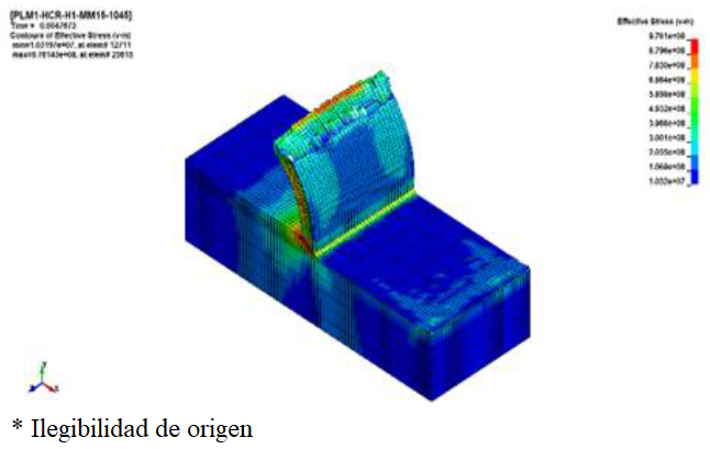
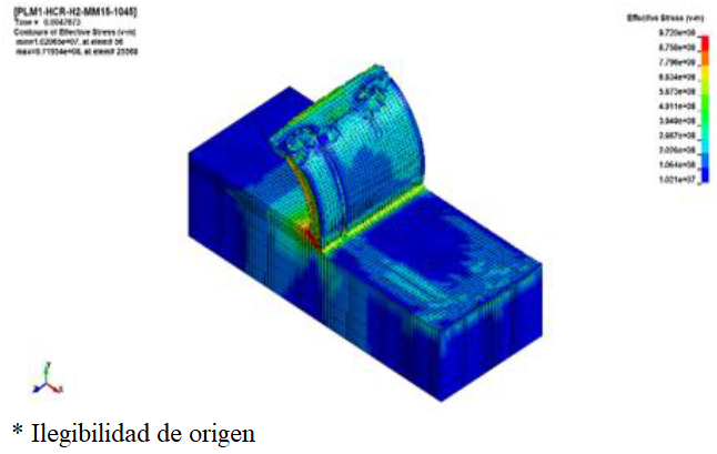
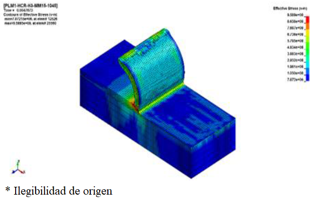
4.7 Chip Generation
From simulations, it can be shown that chip formation is generated and is different for each insert.
Figures 23-25 show the workpiece, edge of tool and chip formation. They are presented showing the Von Mises stress.
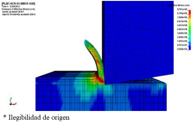
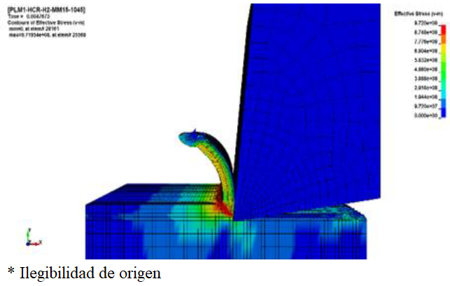
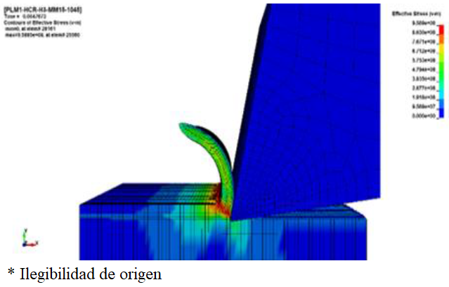
Figures 26-28 shows a close view from chip formation and edge insert. All these figures show the insert in its last position at the end of the simulated time.
5 Conclusions
A model based on finite element theory for orthogonal turning was developed.
Experimental force data were obtained for 0°, 6° and 12° of rake angle carbide insert and those were used to calculate each friction coefficient to feed a Coulomb friction model to solve the contact part between workpiece and tool in LS-DYNA platform.
Johnson-Cook material model was used to define the workpiece behavior without the thermal analysis and assuming low strain rates. It was a structural problem focused on the effect of friction coefficient in simulated cutting forces.
AISI-1045 steel, cold drawn was used to experimental tests, coefficients and parameters for Johnson-Cook material model were taken from literature, leaving the computing of them for further projects.
ANSYS platform was used to generate geometry and mesh for workpiece and inserts, solution was performed using LS-DYNA solver under Windows platform and the results were processed in LS-PREPOST.
For values shown (experimental versus simulated set 1), it can be observed that minimum force difference was 3.61% for insert 1, force difference of 15.91 % for insert 2 and the maximum force difference 32.02% for insert 3. It can be observed (experimental versus simulated set 2) that set 2, behaves like set 1, with the minimum force difference for insert 1, force difference for insert 2 and for insert 3. The values are 3.47%, 15.99%, and 32.02%.
Cutting force and thrust force were obtained from simulations, but thrust force is neglected because edge tool only has horizontal displacement in simulation and the thrust force is computed in the vertical direction (perpendicular to the tool movement) and this is the reason why simulation of insert 1 (0° rake angle, both cases, set 1 and set 2) has a thrust force between 2.2 -2.6 N. For insert 2 (6° rake angle) thrust force was 24 N for both sets. For insert 3 (12° rake angle) thrust force was the maximum value of 48 N for both sets.
It can be concluded from simulated cutting that force behavior it's as expected, whereas rake angle is increasing (0°, 6°, and 12°), cutting force is decreasing (for set 1: 325.64 N, 290.12 N, and 259.40 N; for set 2: 326.12 N, 289.85 N, and 259.40 N; for both sets, values are for inserts 1, 2, and 3 respectively). In the other side, simulated thrust force must have to increase whereas rake angle is increased (for set 1: 2.25 N, 24.05 N, and 48.08 N, for set 2: 2.61 N, 24.28 N, and 48.02 N; for both sets, values are for inserts 1, 2, and 3 respectively).
It can be shown that simulated values (cutting force and thrust force for set 1 and set 2) are almost the same for all the cases even with the use of different friction coefficient (0.85 for all inserts in set 1, and for set 2: 0.7559, 0.8547, and 0.9999 for inserts 1, 2, and 3). From sets comparison, the maximum force difference is 16% for the thrust force (insert 1), and the remaining values were under 0.96%.
Modify friction coefficient doesn't lead to a big difference in reported force values. For insert 1 (for set 1 and set 2 respectively) the friction coefficient was 0.85 and 0.7559 with a difference of 11.07%. For insert 2, values were 0.85 and 0.8547, with a difference of 0.55%, and for insert 3, values were 0.85 and 0.9999, with a difference of 17.64%.
Simulated force gradually increments its value from cero at the beginning of the process, when the insert impacts the workpiece to a steady value when there is chip formation, for the interval 00.001 s. It's more visible for cutting force, though thrust force also presents this behavior. Average values for cutting force were taken from the time interval 0.0015-0.0045 s where cutting process is continuous, and are compared to those from experimental tests taken in the interval 2.5-11.25 s that corresponds to a continuous cutting process.
FEM simulations with tool-workpiece contact, and chip generation are shown. AISI-1045 steel workpiece is setup as deformable body and carbide inserts geometries as rigid bodies.
From data obtained from experimental tests and with the use of equation 2, it can be concluded that keeping feed force and rake angle constant, an increment in experimental cutting force leads to a decrease in friction coefficient; and keeping cutting force and rake angle constants, an increment in feed force leads to an increment in friction coefficient.
Analyzing simulated cutting forces (set 1 and set 2), it can be concluded that an increment in friction coefficient doesn't leads to a noticeable increment in simulated average cutting force for stated conditions.

