


 text new page (beta)
 English (pdf)
 Article in xml format
 Article references
 Send this article by e-mail
 Cited by SciELO
  Similars in
SciELO
Similars in
SciELO 
 Permalink
1 Introduction
Topic models are widely used in text processing and Latent Dirichlet Allocation (LDA) [3] is the core of a large family of probabilistic models. LDA provides an efficient tool to analyze hidden themes in data and helps us recover hidden structures/evolution in big text collections. The key problem in topic models is to compute the posterior distribution of a document given other parameters. The posterior inference problem in topic models is to infer the topic proportion of documents and topics which are distributions over vocabulary. Large datasets or streaming environments contain huge number of documents, hence the problem of estimating topic proportion for an individual document is especially important. The quality of learning for LDA is determined by the quality of the inference method being employed.
Unfortunately, solving directly a posterior distri-bution of a document is intractable [3]. There are two main approaches to tackle it.
One is approximating the intractable distribution by tractable distribution, for example Variational Bayes inference (VB) [3]. The other is a sampling method, which draws numerous the samples from target distribution then estimating the interesting quality from these samples. The well-known method is Collapsed Gibbs Sampling (CGS) [8]. There are also famous methods such as Collapsed Variational Bayes (CVB) [15], CVB0 [2], Stochastic Variational Inference (SVI) [10], etc.
To our best knowledge, there are not any mat-hematical guarantees for quality and convergence rate in existing approaches. Therefore, in practice we do not have any ideas about how to stop the methods we are using but trying, observing and retrying again to reach the best solution.
Another way to solve the posterior distribution is to view it as an optimization problem. To infer about topic proportion of a document is to solve the maximum a posteriori of topic proportion given words in this document and all topics of corpus [16]. This optimization problem is usually non-convex and NP-hard [14]. There is very few theoretical contributions in non-convex optimization literature, especially in topic models. Online Maximum a Posteriori Estimation (OPE) [16] which is an online version of Frank-Wolfe algorithm [9] is a stochastic algorithm to solve such kind of non-convex problem.
OPE is theoretically guaranteed to converge to a local stationary point [16]. Although OPE is easy to implement and has fast convergence and mathematically guaranteed, it remains some problems. The weakness of OPE is that it is not well adaptive with different data sets because of the uniform distribution in its operation. We will exploit this crucial point to propose a new and more general algorithm based on OPE. When changing its operations, we have to retain the advantage of the original algorithms, that is theoretical guarantees.
Our main contribution is following:
— We propose new algorithm called Generalized Online Maximum a Posteriori Estimation (G-OPE) for solving posterior inference problem in topic models. G-OPE is more general and flexible than OPE, adapts better in different datasets and preserves the key advantages OPE.
— We employed G-OPE into the existing algorithm Online-OPE [16] to learn LDA in online settings and streaming environments.
— We conduct experiments to demonstrate that Online-GOPE outperforms existing methods to learn LDA.
Organization: The rest of this paper is organized as follows. In Section 2, we introduce an overview of posterior inference with LDA and main ideas of existing methods. In Section 3, our new algorithm G-OPE is proposed in details. In Section 4, we conduct experiments with two large datasets with state-of-the-art methods in two different measures. Finally Section 5 is our conclusion.
Notation: Throughout the paper, we use the following conventions and notations. Bold faces denote vectors or matrices. x
i
denotes the i
th
element of vector x, and A
ij
denotes the element at row i and column j of matrix A. The unit simplex in the n-dimensional Euclidean space is denoted as
2 Related Work
LDA [3] is the basic and famous model in topic modeling. It models each document as a probability distribution θ d over topics, and each topic β k as a probability distribution over words. In Fig. 1, K is number of topics, M is number of documents in corpus, N is number of words in each documents.

Note that θ d ∈ ∆ K , β k ∈ ∆ V . The generative process for each document d is as follows:
The most important problem we need to solve in order to use LDA is to compute the posterior distribution p(θ, z|w, α, β) of hidden variables in a given document d. However, it is intractable. There are many ways to handle it. Variational Bayesian Inference [3] approximates p(z d , θ d , d|β, α) by obtaining a lower bound on the likelihood which is adjustable by variational distributions. CVB and CVB0 deal with p(z d , d|β, α), CGS draws samples from p(z d , w|β, α) to estimate it. Eventually, all methods try to estimate the topic proportion θ d .
In this paper, we infer topic proportion for a document directly by solving the Maximum a Posteriori Estimation (MAP) of θ d given all words of this document and parameters of the model. The MAP estimation of topic mixture for a given document d:
using Bayes’ rule, we have:
Under the assumption about the generative process, problem (2) is equivalent to the following:
Within convex/concave optimization, problem (3) is relatively well-studied. In the case of α ≥ 1, it can easily be shown that the problem (3) is concave, and therefore it can be solved in polynomial time.
Unfortunately, in practice of LDA, the parameter α is often small, says α < 1, causing problem (3) to be non-concave. Sontag et al. in [14] has showed that problem (3) is NP-hard in the worst case when parameter α < 1. Consider problem (3) as a non-convex optimization problem, the gradient-based methods such as Gradient Descent (GD) and its variants are ineffective because of the existence of saddle points and flat regions, hence we need an effective random method to avoid them. OPE [16] is an efficient iterative algorithm for solving problem (3). It is a good solution in escaping saddle points and flat regions.
In the literature of iterative optimization algorithms, in each iteration, they try to build a tractable function that approximates true objective function, then optimize approximating function to reach the next point. The various algorithms have different techniques to build their own approximation. For example, using Jensen’s inequality, Expectation-Maximization (EM) [5] or Variational Inference (VI) [3] calculate the Evidence Lower Bound (ELBO) then maximize it. Gradient Descent constructs its quadratic approximation in each step and minimizes the quadratic. OPE solves the problem (3) by constructing an approximate sequence by stochastic way and solve it by Frank-Wolfe update formula [7].
Details of OPE is in Algorithm 1. The idea of OPE is quite simple. At each iteration t, it draws a sample function f t (θ) and builds the approximation F t (θ) which is the average of all previous sample function. The most interesting idea behind OPE is that the objective function is the sum of a likelihood and a prior. In each step, it builds an approximate function F t (θ) by choosing either likelihood or prior with equal probabilities {0.5, 0.5}. That means when inferring about the topic proportion of a document, we use either the evidence of the document (likelihood) or knowledge we have known before (prior). This behavior is very natural to human. However, OPE considers likelihood and prior with the same contributions by using uniform distribution.

In fact, when humans deal with a new sample, one can rely on more likelihood if we have observed enough evidences, or rely on more prior knowledge if we have been lack of evidences. This simple idea leads us to build a more general and flexible version of OPE by using Bernoulli distribution instead of uniform distribution.
3 Generalized Online Maximum a Posteriori Estimation
In this section, we introduce our new algorithm, namely Generalized Online Maximum a Posteriori Estimation (G-OPE) based on OPE. OPE operates by choosing the likelihood or prior at each step t, then builds the approximation F t (θ) which is the average of all parts draw from previous steps and current step. In G-OPE, in order to introduce the Bernoulli distribution into the sampling step, we need to modify the likelihood and prior so that the approximation function F t (θ) → f(θ) as t → ∞. Denote:
then the true objective function f(θ) includes two components:
where g 1(θ) and g 2(θ) are the log likelihood and prior respectively.
Denote:
where G 1(θ) and G 2(θ) are the adjusted likelihood and prior respectively.
G-OPE is detailed in Algorithm 2. In Algorithm 2, f(θ) is the true objective function we need to maximize. At t th iteration, we draw sample function f t (θ) from set of adjusted likelihood G 1(θ) and prior G 2(θ), then we build the approximate function F t (θ). Because G-OPE is stochastic, in theory we consider T → ∞, where T is number of iterations for whole algorithm.
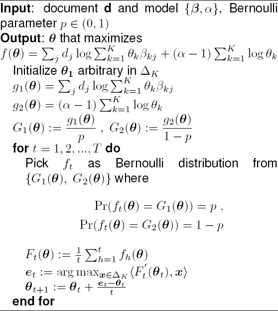
We use Bernoulli distribution with parameter p to replace for uniform distribution in OPE. At t th iteration, we pick f t (θ) as Bernoulli random variable with probability p from {G 1(θ) , G 2(θ)} where:
In statistic theory, as t increases (at least 20) and it is better to choose p not close to 0 or 1. Consider t independent Bernoulli trials with probabilities:
we build a stochastic approximate sequence:
We find out that F t (θ) is the average of all sample functions drawn until current step.
So it is guaranteed to converge to f(θ) as t → ∞, which will be shown in Theorem 1. The Bernoulli parameter p controls how much likelihood part and prior part contribute to the objective function f(θ). We can utilize this point to choose the most suitable p in each circumstance. OPE is a special case of G-OPE when Bernoulli parameter p is chosen equal to 0.5. So OPE is not flexible in many datasets. G-OPE adapts well with different datasets, we will show it in the experiment section. In the rest of this section, we will show that G-OPE preserves the key advantage of OPE which is the guarantee of the quality and convergence rate. This character is unknown for the existing methods in posterior estimation in topic models.
Theorem 1 (Convergence of G-OPE algorithm)
Consider the objective function f(θ) inEq. 3, given fixed d, β, α, p. For G-OPE, with probability one, the followings hold:
1. For any θ ∈ ∆ K , F t (θ) converges to f(θ) as t → +∞.
2. θ t converges to a local maximal/stationary point of f(θ).
Proof: Before the proof, we remind some notations: B(n, p) is binomial distribution with parameters n and p (Bernoulli distribution is a special case of the binomial distribution with n = 1), N(µ, σ 2) is normal distribution. E(X) and D(X) are expectation and variance of random variable X respectively.
We find out that problem 3 is the constrained optimization problem with the objective function f(θ) is non-convex. The criterion used for the convergence analysis is importance in non-convex optimization. For unconstrained problems, the gradient norm
Denoted:
and
so,
Pick f
t
follows the Bernoulli distribution from
Let a t and b t be the number of times that we have already picked G 1(θ) and G 2(θ) respectively after t iterations.
We find that a t + b t = t or b t = t − a t . We have a t ∼ B(t, p) and E(a t ) = t.p , D(a t ) = t.p.(1 − p).
We have:
where S t = a t − t.p.
We have:
then S t → N(0, tp(1 − p)) when t → ∞.
So S t /t → 0 as t → ∞ with probability one. From (4), we conclude that the F t → f as t → +∞ with probability one.
Consider:
Note that g
1(θ), g
2(θ) are Lipschitz continuous on
We have:
Since e
t
and θ
t
belong to
Therefore, there exits a constant c 1 > 0 such that:
Summing both sides of (5) for all t, we have:
As t → +∞, f(θ t ) → f(θ*) due to the continuity of f(θ). As a result, (6) implies:
Note that
So
Because
If exists
Since
Besides, in the non-convex optimization field, the idea of how to build the approximate function in G-OPE can be utilized in the case of objective function f which is the sum of two parts f = g + h. In each step, choose g or h in Bernoulli distribution with parameter p, and adjust p to adapt with different circumstance. Randomness can help algorithms jump out of local minimum/maximum.
Therefore, to design new stochastic algorithms, we begin with a deterministic version, add a sequence of approximation in the G-OPE style, working with each approximation at each iteration by deterministic update formula. This is an open idea for our future works.
4 Experiments
In this section, we will investigate the performance of G-OPE in real world datasets. G-OPE can play as the core inference step when learning LDA, we will investigate the performance of G-OPE through the performance of Online-OPE [16] when changing its core inference method. So we derived Online-GOPE.
We conducted two experiments. The first one is the effect of parameter p in G-OPE when learning LDA and the second is in comparison Online-GOPE with the current state-of-the-art methods.
4.1 Datasets and Settings
The datasets for our investigation are New York Times and Pubmed1. These are very large datasets. The number of documents is large and the size of vocabulary is large also. Details of datasets are presented in Table 1.
Table 1 Two data sets for our experiments
| Data sets | No.Documents | No.Terms | No.Train | No.Test |
| New York Times | 300000 | 141444 | 290000 | 10000 |
| Pubmed | 330000 | 100000 | 320000 | 10000 |
To evaluate the performance of learning methods in LDA, we used Log Predictive Probability (LPP) and Normalized Pointwise Mutual Information (NPMI) measures. These measures is commonly used in topic models. Predictive Probability [10] measures the predictiveness and generalization of a model to new data, while NPMI [1, 4] evaluates semantics quality of an individual topic in these models.
Some common parameters is set as follows: the number of topics is K = 100, the hyper-parameters in LDA model is
As algorithms we compares are stochastic, so to avoid randomness, we run each method five times, and report the average results.
The script of experiments is that: for the first experiment, we run Online-GOPE with different values of parameter p then choose the best one. In the second experiment, we compare Online-GOPE obtained with the best parameter p to some methods in learning LDA such as VB, CVB, CGS, OPE.
4.2 The Effect of Bernoulli Parameter p
In this experiment, we investigate how important the value of parameter p is. Because p ∈ (0, 1), and p is good if it is not close to 0 and 1. So we choose p respectively in {0.1, 0.15, ..., 0.9}, then run Online-GOPE in two datasets. We report the performance of Online-GOPE in Fig. 2 and Fig. 3. We can easly observe that p affects very much in the performance in terms of both measures. In Fig. 2, Online-GOPE reaches the best performance on New York Times for LPP measure at p = 0.35 and for NPMI measure at p = 0.75. In Fig. 3, Online-GOPE reaches the best performance on Pubmed for LPP measure at p = 0.4, for NPMI measure at p = 0.45.
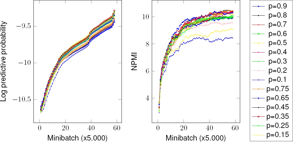
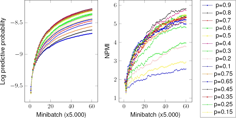
This results support our idea about the contributions of likelihood part and prior part of topic proportion inference for a document. The different dataset has the suitable value of p. If we want to get the best performance on the generalization or on semantics quality of topics, we have different p to choose. Therefore G-OPE is very flexible in the real world dataset.
The good values of p depend on how much likelihood part and prior part possess in total. The likelihood depends on the length of the documents. In our datasets, the average length of a document in New York Times is 329 while the average length of a document in Pubmed is 65. That explains why we have different best values of p for each dataset.
4.3 Comparison of G-OPE with Novel Algorithms
In this experiment, we compare Online-GOPE with the best value of p in previous experiment to the original Online-OPE and other methods: Online-VB, Online-CVB, Online-CGS. All of these algorithms try to learn the topics over the words β or variational parameters λ. The difference among these algorithms is the inner inference procedures.
The results is shown in Fig. 4 and 5. With suitable parameter p, we obtained G-OPE which was better than OPE, VB, CVB, and CGS on LPP measure. For NPMI measure, all algorithms perform the same, but G-OPE is one of the tops.

Fig. 4. Online-GOPE compares with Online-OPE, Online-VB, Online-CVB and Online-CGS on New York Times dataset. Higher is better

Fig. 5. Online-GOPE compares with Online-OPE, Online-VB, Online-CVB and Online-CGS on Pubmed dataset. Higher is better
This results show that Online-GOPE performs better than not only original OPE, but also the current novel methods. G-OPE works well because of the right choose of controlled parameter p.
5 Conclusion
We have discussed how posterior inference for individual texts in topic models can be done efficiently with our method. In theory, G-OPE remains the guarantee on quality and convergence rate of original OPE algorithm, which is the most important character among existing state-of-the-art inference methods. In practice, the parameter p of Bernoulli distribution in our method is a flexible way to deal with different datasets.
Besides, the spiritual idea in building approximation functions from G-OPE can be easily extended to a wide class of maximum a posteriori estimation or non-convex problems. By exploiting G-OPE carefully, we have derived an efficient method Online-GOPE for learning LDA from data streams or large corpora. As a result, it is the good candidate to help us to work with text streams and big data.
6 Predictive Probability
Predictive Probability shows the predictiveness and generalization of a model M on new data.
We followed the procedure in [12] to compute this measurement. For each document in a testing dataset, we divided randomly into two disjoint parts w obs and w ho with a ratio of 80:20. We next did inference for w obs to get an estimate of 𝔼(θ obs ). Then we approximated the predictive probability as:
where
7 NPMI
NPMI measurement helps us to see the coherence or semantic quality of individual topics. According to [11], NPMI agrees well with human evaluation on interpretability of topic models. For each topic t, we take the set {w 1, w 2, . . . , w n } of top n terms with highest probabilities. We then computed:
where P (w i , w j ) is the probability that terms w i and w j appear together in a document. We estimated those probabilities from the training data. In our experiments, we chose top n = 10 terms for each topic. Overall, NPMI of a model with K topics is averaged as:

