


 text new page (beta)
 English (pdf)
 Article in xml format
 Article references
 Send this article by e-mail
 Cited by SciELO
  Similars in
SciELO
Similars in
SciELO 
 Permalink
1 Introduction
Nowadays, the design of chemical processes must to consider not just delivering products of high quality, but also performing this task with minimum both energy requirements and environmental impact. According to Yue et al. [30], “concerns about climate change, waste pollution, energy security, and resource depletion are driving society to explore a more sustainable way for development and manufacturing” [30]. In order to design chemical processes with the minimum energy requirements several researches have been focus their efforts in the development of optimization strategies; these strategies include mathematical programming [1, 26, 19, 5, 22, 9, 31] or stochastic techniques [18, 20, 28, 24, 32, 23]. Regardless the optimization technique used, it is necessary a model of the chemical process. Some works employ reduced models, which are more simple and easy to implement; another strategies consider complete models, usually linking the optimization strategies to chemical processes simulators. Next, we give a brief review of some works that consider the last approach, for different purposes.
Lababidi et al. [17] developed a prototype design support system for process engineering, in order to analyze the controllability and dynamics of process during the conceptual design stage. They integrated MATLAB® with Omola®, through object-oriented message passing to get this objective.
Later, Ramzan & Witt [25] proposed a methodology for decision support among conflicting objectives; for this, they used a multiobjective optimization layer based on goal programming using Aspen Plus® and the optimization tool for MATLAB®.
In 2008, Tona Vásquez et al. [27] presented an approach to realize multiscale modeling for the production of perfume microcapsules.
Their strategy connects modules developed in MATLAB® with the operation models developed in Aspen Plus®. Gutiérrez-Antonio and Briones-Ramírez [12] proposed the use of a multiobjective genetic algorithm with constraints handling for the optimization of Petlyuk sequences. The optimization tool, developed in MATLAB®, is coupled to Aspen Plus® in order to get the information of the objectives and constraints required. In 2011, Khodadoost and Sadegui [15] reported a dynamic simulation study of distillation column sequences in a Gas Refinery. They linked the module Dynamics of Aspen Plus® and MATLAB® Simulink® software to perform their work. In the same year, Eslick and Miller [8] reported a work where the freshwater consumption was minimized; the study case was a pulverized coal power plant with a capacity of 550 MW. Their framework uses an optimization scheduler, based on NSGA-II [7], which is linked to Aspen Plus® by means of Excel®. In addition, Alabdulkarem et al. [2] optimized the propane pre-cooled mixed refrigerant of a liquefied natural gas plant. In order to realize the optimization, they used a genetic algorithm, taken from the MATLAB® optimization toolbox, along with a computer model in Aspen HYSYS®. Bhattacharyya et al. [3] made a study of the control performance during load, following in a coal-fed integrated gasification combined cycle power plant. They developed a steady-state model, which was exported to the module Dynamics of Aspen Plus®, and integrated with MATLAB®. In the same year, Kiss et al. [16] proposed a novel biodiesel process based on a reactive dividing wall column. As a design tool, they used simulated annealing as optimization technique, which was coupled to Aspen Plus® through Excel®.
From the previous works, it is clear that the linkage of a processes simulator is very useful; since it allows considering the complete model of the chemical processes, taking advantage of the complete thermodynamic properties data base of the processes simulator. Nevertheless, none of the above works have presented detailed information on how to make the link of MATLAB® with the process simulator directly, Aspen Plus®. The availability of this procedure allows the use of complete models for the chemical processes, taking advantage of all the modeling capabilities of the process simulators, no matter the kind of optimization technique used.
Thereby, in this work we propose a procedure to perform the link between MATLAB® and Aspen Plus® processes simulator. We present the information requirements, information flows and the communication commands. Also, instructions to generate automatically the bkp files of the optimal designs are presented.
2 Selection of the Chemical Process
In this section, we present the first step required to perform the optimization rigorously, which is the selection of the chemical process. For the selected chemical process, we have to choose the objectives to optimize, and the constraints involved, if they are any. The objectives and/or constraints are the information that guides the optimization process, and also it is the information that is generated in the simulation of the chemical process in Aspen Plus®.
In addition, we must to list the process variables required for the simulation; with this information objectives and/or constraints can be calculated in the simulation. These variables are manipulated in the optimization strategy. It is desirable to record variables, objectives and constraints as vectors in a database; this will allow having all the required information of the optimal solution.
Thus, the problem statement can be established as:
3 Procedure to Link MATLAB® and Aspen Plus®
In this section, the linking procedure is presented. In order to illustrate this procedure, we will use a multiobjective genetic algorithm with constraints’ handling written in MATLAB® [12]; however, the procedure can be used with any other optimization technique, considering or not constraints.
The details of the multiobjective optimization strategy can be consulted in a previous contribution [12].
Figure 1 shows the general procedure of the link between MATLAB® and Aspen Plus®.
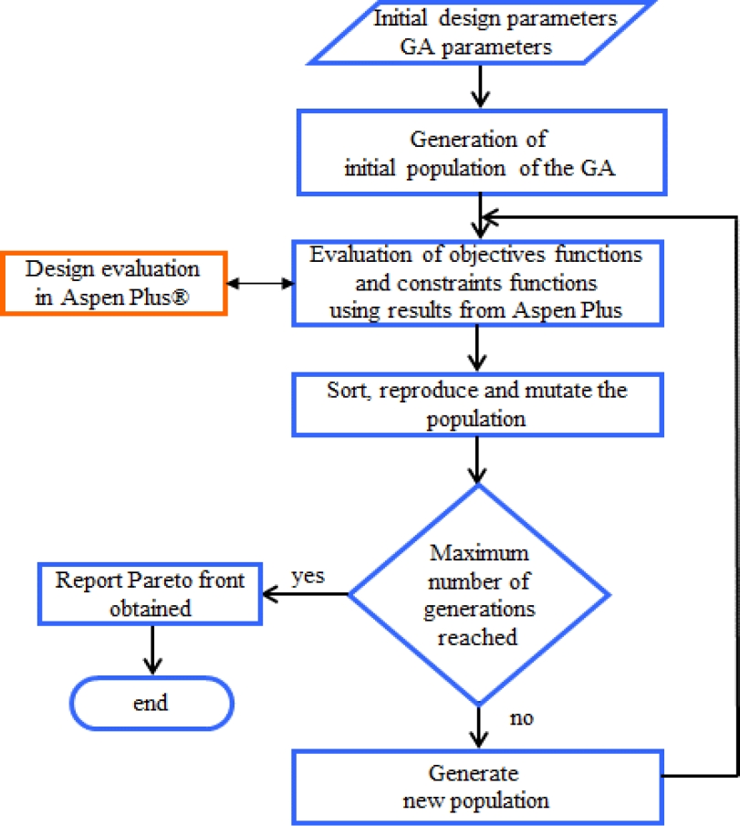
According to Figure 1 we can observe that the first step is giving the initial design parameters of the chemical process, information that was presented in section 2. In addition, the parameters of the optimization strategy must be defined. With this information the optimization strategy begins with the generation of the initial population. The entire population is composed of individuals, which are sent one by one to Aspen Plus® in order to be evaluated in terms of objectives and constraints. Once all individuals are evaluated the optimization strategy can continue with the sort, reproduction and mutation steps. If the maximum number of generations is reached, then the optimization strategy reports the Pareto front; otherwise, the procedure continues until that criterion is satisfied.
On the other hand, the Figure 2 shows the details of the Design evaluation in Aspen Plus® orange block. As can be seen, the first step is that MATLAB® sends the instruction to open Aspen Plus®; after that, MATLAB® sends to Aspen Plus® the required information to perform the simulation, and the instruction to perform the simulation is also sent. Once the simulation has been performed, MATLAB® takes back the results of the objectives and constraints, in order to be fed to the optimization strategy.
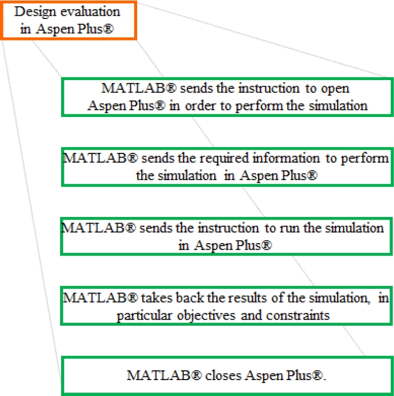
Finally, MATLAB® sends the instruction to close Aspen Plus®, in order to reduce the use of RAM memory. In the present contribution, the details of how to perform the operations presented in Figure 2 are given, considering a study case for illustrative purposes. It is worth to mention that this procedure was developed with MATLAB® 2007 and Aspen Plus® V7.1, and the code was validated from these versions until MATLAB® 2012 and Aspen Plus® V9.1. However, the instructions can be applied to further versions if the main core of instructions of both software does not change.
Before entering to the detailed instructions of the operations showed in Figure 2, we need to create a file with the simulation of the process of interest in Aspen Plus®. Usually, this file is saved with extension apw; however, the file employed in the linking process is the one with extension bkp. In the simulation file, it is desirable that the names of the blocks and streams follow a logic methodology; this is especially useful in complex chemical processes, and also it helps to the standardization of the optimization code for future cases.
Also, we recommend ordering the components according with the decreasing relative volatility. It is important to initialize the recycled streams (if there are any), i.e. interconnection or recycle flows; this will help to improve the convergence of the schemes where recycle streams are presented.
We are going to illustrate the process with a Petlyuk sequence, which is showed in Figure 3. We consider that we are interested in minimizing the number of stages in prefractionator, NSTAGE_B1, the number of stages in main column, NSTAGE_B2, and the heat duty in main column, DUTY. The constraints are the recoveries of the three components presented in the feed stream.
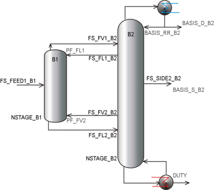
In order to perform this optimization, we manipulate 12 variables which are: feed stage in column B1 (FS_FEED_B1), number of stages in column B1 (NSTAGE_B1), reflux ratio in column B2 (BASIS_RR_B2), number of stages in column B2 (NSTAGE_B2), distillate stream flow of column B2 (BASIS_D_B2), side stream flow of column B2 (BASIS_S_B2), product stage of liquid interconnection flow FL1 in column B2 (FS_FL1_B2), feed stage of vapor interconnection flow FV1 in column B2 (FS_FV1_B2), vapor interconnection flow (PF_FV2), feed stage of liquid interconnection flow FL2 in column B2 (FS_FL2_B2), product stage of vapor interconnection flow FV2 from column B2 (FS_FV2_B2), and the liquid interconnection flow (PF_FL1).
As was mentioned before, we have to identify the objectives and/or constraints of the optimization problem, along with all involved variables, manipulated and required for the simulation.
The objectives, constraints and manipulated variables are vectors, as described next.
The variables presented in Algorithm 1 represent the initial values for the optimization strategy. Nevertheless, in all optimization strategies, new values have to be generated for all variables that are manipulated and fed to Aspen Plus® to perform the simulation.

These variables must be declared in the optimization code, and they will be used to assign the values from MATLAB® into the simulation file in Aspen Plus®:
It is worth to mention that NameVark represents the vector of variables that are manipulated during the optimization strategy.
At this point, we have identified objectives, constraints, manipulated variables and required variables for the simulation in Aspen Plus®, which file has already been created; also, the values generated by the algorithm are declared and stored for its posterior use. Now, the following step is opening Aspen Plus® from MATLAB®.
We initiate this process by giving to MATLAB® the route where the bkp file, that contains the process is located, and also we give some instructions to delete all files that Aspen Plus® could generated in a previous simulation.
This procedure is shown in Algorithm 3.


The code instructions shown in Algorithm 3 assign the route to a string type variable. We use a virtual disk where the old files are deleted in order to avoid conflicts; nevertheless, you must to use your personals options in drive letters and routes.
Thus, the file of name ' strColType ' ' strMezcla '.bkp' is located in the Folder strMezcla, inside the Folder strColType, inside the Folder 2, which is located in Folder 1.
The information after the sign % are comments, while the rest are the code lines. In this work, we are going to use Aspen Plus® as a local OLE automation server [6]; in other words, we are going to manage Aspen Plus as an external subroutine that allows to generate the values of objectives and constraints required in the optimization strategy.
In this case 'Apwn.Document' is the programmatic identifier of an OLE-compliant COM server, and h is the handle of the server's default interface.
It is worth to mention that in MATLAB® a handle is a reference to an object. Then, the following instruction (Algorithm 4) opens Aspen Plus® from MATLAB® along with the simulation of interest.

In the previous instructions, in Algorithm 4, ihAPsim variable is the handle of the server. Also, the instruction refers to opens strFileAspen, which is the file specified in Algorithm 3.
In this routine, we use a variable from the class ihNode from the automation server; in this object, Aspen Plus® expose the problem input a result data as a tree structure composed of ihnode objects. The used subroutine navigate across the tree structure of variables in Aspen Plus® until find the last node of the variable name, where the “value” method is used to recall the value; when the last node is an array, the subroutine recall the value of the element in the array. Also, the subroutine performs some validation, but for the complexity of the tree of Aspen Plus® the user must to be sure that the names are correct; otherwise the subroutine ends with an error message.
Once the simulation is open, the names of the compounds used in the simulation are retrieved along with the flow of the main stream of the process in the flowsheet (see Algorithm 5).

In Aspen Plus®, every simulation flowsheet has different names thereby we need to program separated functions for each process. In order to make the code more generic we use a handle to change the unit operations of the process.
The handle for each type of process flowsheet is generated with the code showed in Algorithm 6. The instructions to modify the processes variable are contained in this handle, and it will be presented later. At this point, we can make a simulation with the instructions included in Algorithm 6. Each one of the functions for different process has the next structure. The input arguments are: Solution: an array with the values of the manipulated variables in Aspen Plus®, like number of stages, stream flows, among others; ihAPsim: is the handle of the Aspen Plus® server, with the corresponding bkp file opened. And the output arguments are: SolutionFactibility: return true if the solution is feasible (for instance that the total number of stages is greater than the number of the feed stage); SolConstraints: returns the value of the variables defined as constraints (recoveries in this example); Objectives return the value of the variables defined as objectives (number of stages and heat duty in this example). When the simulation is finished and the interested values are retrieved, we can Close Aspen Plus® and it releases the resources in MATLAB®.

On the other hand, the handle subroutine allows modifying the values of the variables required to perform the simulation in Aspen Plus®. Thereby, we start the process of assigning names for all variables in Petlyuk sequence: prefractionator, main column, product and interconnection stream flows, along with some string assignations required to retrieve the values of composition in each product stream (see Algorithm 7).

Before sending these values to Aspen Plus®, we suggest to perform a feasibility verification of the values of the variables; this verification is focused in the physical meaning of the variables. In this way, the variables sent to Aspen Plus® are consistent or physically feasible.
For instance, in the prefractionator the feed stage number must be minor or equal to the total number of stages, but never bigger, and also greater to zero. This can be expressed as is shown in Algorithm 8. The next step is reinitiating the simulation before the values are changed in Aspen Plus®; this is required to have reliable results on the convergence of the simulation (see Algorithm 9).


Once that the values are assigned to the variables, these must be sending to Aspen Plus® to perform the simulation. In order to do this, we have created other subroutines to simplify the connection to Aspen Plus®. The subroutine SetValueAspenVariable is used to write a value to a variable in Aspen Plus®. The function to call this subroutine is shown in Algorithm 10.
Where the input arguments are: strVariable: string with the name of the variable to read, as appear in the Variable Explorer option, inside the Tools Menu of Aspen Plus®; ValAspen: value to be written in the strVariable of Aspen Plus®; ihAPsim: object of type ‘Apwn.Document’ successfully initialized with a valid Aspen Plus® bkp file. And the output arguments are: Varargout: funOk MsgAspen; funOk: boolean value indicating a succesfully read; MsgAspen: error message displayed from Aspen Plus® when a variable cannot be read.
In this routine, we use a variable from the class ihNode from the automation server; in this object, Aspen Plus® expose the problem input a result data as a tree structure composed of ihnode objects.
The used subroutine navigate across the tree structure until find the last node of the variable name, where the “value” method is used to recall the value; when the last node is an array, the subroutine recall the value of the element in the array. Also, the subroutine performs some validation, but for the complexity of the tree of Aspen Plus® the user must to be sure that the names are correct; otherwise the subroutine ends with an error message.
Next, we have to set the value of all manipulated and required variables inside Aspen Plus® file to perform the simulation. All route variables can be found in the Variable Explorer option, inside the Tools Menu of Aspen Plus®. Then, we begin changing values of variables in the prefractionator, main column, along with product flows (see Algorithm 11).

Once all required and manipulated variables are sent to Aspen Plus®, then the simulation is performed with the following instructions (Algorithm 12).

Another subroutine developed to simplify the code is VerifyRunStatusError, which is executed as follows (Algorithm 13).

In this function, we read the error matrix of Aspen Plus® in case that it exists, which is located in the following path: 'Application.Tree.Data. ResultsSummary.Run-Status.Output. PER_ERROR.Elements'. If this matrix does not exist, then the simulation has a successfully end, and we accept to the results of the performed simulation.
As was mentioned before, we have created several subroutines in order to simplify the connection to Aspen Plus®. For instance, GetValueAspenVariable is used to read a variable from Aspen Plus® simulation file, and it is used as follows (Algorithm 14):

Where the input arguments are: strVariable: string with the name of the variable to read, as appear in the Variable explorer menu from Aspen Plus®; ihAPsim: object of type ‘Apwn.Document’ successfully initialized with a valid Aspen Plus® bkp file. The output arguments are: ValAspen: value of the requested variable; Varargout: funOk MsgAspen; funOk: boolean value indicating a succesfully read; MsgAspen: error message displayed from Aspen Plus® when a variable cannot be read. This subroutine is very useful to take back the information from Aspen Plus® to MATLAB®.
At this point, Aspen Plus® has simulated the process, and we have three possible scenarios with respect to the convergence: convergence without warnings, convergence with warnings and no convergence due to errors. If the simulation converges and there are available results, with or without warnings, then the values of objectives and constraints of interest are taken back to MATLAB®, using these commands (Algorithm 15).

If the simulation does not converge, then the algorithm allocates infinite heat duty and purities and recoveries of zero. Once that the objectives and/or constraints values are taken back to MATLAB®, the optimization process can continue. We suggest using a data base to record all the values of manipulated variables, objectives and/or constraints; so, all the information of the performance of the optimization strategy and final results are available any time.
The main advantage of using a database if there is not storing limit, in counterpart with the limitation in the number of cells found in Excel®. Also, the direct relation between MATLAB® and Aspen Plus® avoid losing information; for instance, when the connection is through Excel®, this software can crash and all the information will be missing. Also, the use of database allows having data processing tools, or even this database can be used for data mining. It is worth to mention that this software has been used to the study of different types of chemical processes with interesting results [29, 4, 13, 21, 11, 14, 10].
4 Generating bkp Files of Optimal Solutions
Once than the optimization procedure has been performed, we have as results a single or a set of optimal designs; depending if we are using a mono or multi objective strategy.
Thus, it would be desirable to generate automatically the bkp files for all optimal solutions, in order to analyze composition, temperature or pressure profiles, or even use them to generate dynamic files and performing control studies. Next, the procedure to generate bkp files, given a set of design variables for n optimal designs, is presented.
First, we need to create a matrix in MATLAB® where each row represents a complete design of a given process, and the columns represent a variable of each design:
Once that the matrix is created the following code is executed. First, the size of the matrix is determined (30) (see Algorithm 16).

Then, we initialize a counter, and the handle function is generated according with the type of process. This handle denotes the name of the process or unit operations whose optimal solutions bkp files are going to be generated (see Algorithm 17).

Next, Aspen Plus® is open with the following instructions (Algorithm 18).

Once Aspen Plus® is opened, then we use a cycle to simulate and save each optimal design, with the following code (Algorithm 19):
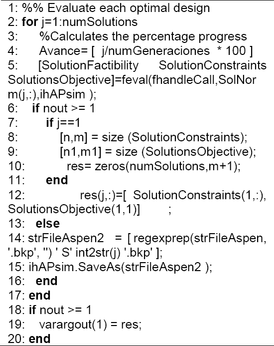
Finally, Aspen Plus® is closed and the resources are released (see Algorithm 20).

The files generated are going to be located in the same folder where the original file for the optimization is located. The name of the file will be the same of the process type, plus the identification code S1, S2, …, Sn designs, where Sn refers to the nth solution.
5 Conclusion
A procedure to link Aspen Plus® with MATLAB® has been presented, including the generation of bkp files of optimal designs. The link between these two powerful tools has great value, since it allows using the computational capabilities of MATLAB® along with the complete models for chemical process of Aspen Plus®. The main advantage of this link is the reduction in computational resources, since just two softwares are running, and the storage capacity of all generated solutions is not limited, as in the case where Excel® is used as linking software. The availability of this code allows increasing the use of complete models in the optimization of chemical processes.

