


 text new page (beta)
 English (pdf)
 Article in xml format
 Article references
 Send this article by e-mail
 Cited by SciELO
  Similars in
SciELO
Similars in
SciELO 
 Permalink
1 Introduction
To reduce in a significant way, the probability of collapse of buildings due to the presence of strong ground motions, the buildings must be designed or retrofitted according to modern seismic codes. However, these codes are made considering a different type of information. For instance, the people that update a seismic code usually use the results of Probabilistic Seismic Hazard Assessment (PSHA) to define basic values of acceleration that must be used as a part of the seismic design of buildings. In some cases, the seismic codes include as a requirement the performing of a specific PSHA to design important structures.
A significant advantage of the PSHA is that it allows considering important uncertainties that are related to the earthquake phenomenon, for instance, the uncertainties related to the number of earthquakes that can occur in a site or the uncertainties related to the maximum earthquake that can be originated in a seismic region. In summary, the results of a PSHA depends on numerous variables with important levels of uncertainties related. Due to this complexity, it is convenient to execute sensitivity analysis. The sensitivity analyzes are procedures that usually offer complementary information to the procedures to perform PSHA. For instance, in general, the results of sensitivity analysis can be applied to support decisions during a PSHA.
At the same time, those results can be helpful during the interpretation stage of the results of the PSHA. In the city of Barcelona co-exist, the Football Club Barcelona, one of the most important football soccer teams of Europe, and the Marenostrum 4 [7], one of the most powerful supercomputers of Europe. The owners of the Football Club Barcelona must have interest in to know the answers to questions as the following:
Can occur some seismic ground motion in Barcelona that can produce significant damage to the Camp Nou stadium? Which is the probability of occurrence of a value of Peak Ground Acceleration (PGA) that can produce some damage to the Camp Nou stadium? Which is the probability that significant damage can occur in the Camp Nou due to a seismic ground motion? Which is the probability of occurrence of the different levels of damage in the Camp Nou?
Similarly, the authorities of the BSC also must have the necessity to know the answer to analogous questions to determine: a) the levels of seismic hazard for the site where the building that contains to the Marenostrum 4 is located and; b) the levels of seismic risk for the building where the Marenostrum 4 is located.
The knowledge of the levels of seismic hazard and seismic risk are fundamental data to make informed decisions about the safety of the Camp Nou, and the Chapel where the Marenostrum 4 is located. With a comparable idea, it is convenient to know the levels of seismic risk of all the buildings of cities as important as Barcelona. In the present study, we did a sensitivity analysis associated with the seismic hazard of Barcelona, which is the most important city of Catalonia. In this study, the sensitivity analysis that we performed had the purpose of contributes to determining the influence of different variables used as data, in the results of seismic hazard. For this reason, in the present document, we described the main features of a sensitivity analysis related to the PSHA for Barcelona. As a part of this analysis, we performed PSHA for various cases. For this last purpose, we applied the new R-CRISIS [21], which is the updated version of the code CRISIS2015 [2,20].
We notice that the sensitivity analysis of the present study was oriented to identify the influence of three variables on the results of the seismic hazard of Barcelona.
These variables are the following: a) the relationship magnitude-macroseismic intensities; b) the beta parameter that defines part of the seismicity of the seismic sources and; c) the ground motion prediction equations (GMPEs). To describe in detail the sensitivity analysis we divided this paper into four sections: 1) introduction; 2) sensitivity analysis for the PSHA of Barcelona (methodology and data); 3) results of the sensitivity analysis for the PSHA of Barcelona and; 4) conclusions. This paragraph is part of section1. In section 2, we described the methodology and the main data applied to perform the sensitivity analysis. In section 3, we included the main results obtained from the sensitivity analysis. And finally, in section 4, we mentioned the main conclusions determined according to the results of the sensitivity analysis. For instance, the results show that the magnitude-intensity macroseismic relationship and the Ground Motion Prediction Equation (GMPE) have a significant influence on the seismic hazard results for Barcelona.
2 Sensitivity Analysis for the PSHA of Barcelona: Methodology and Data
We chose the probabilistic approach of Esteva and Cornel [8, 9] to perform the computation of the different PSHA. Particularly, we used the new R-CRISIS [21] that is based on an updated version of the probabilistic approach of Esteva and Cornel to assess seismic hazard. This approach is summarized in Eq. (1):
is a specific value of A; γ(A*) is the annual frequency of exceedance of A* due to the earthquakes that can occur in the seismic sources;
On the other hand, significant validation of R-CRISIS has already been done [18, 22]. R-CRISIS is a standalone software that works on the operative system Windows, and it is a freeware software that is available on the website of R-CRISIS (http://www.r-crisis.com/).
To perform the sensitivity analysis for the PSHA of Barcelona, we applied R-CRISIS and followed a procedure based on the following steps: A) determination of the main data that will be used to compute the seismic hazard; B) proposal of the different cases that will be considered to perform PSHA. We defined these cases in function of the main variables that we studied in the sensitivity analysis; C) performing of the PSHA for each case; D) analysis of the results of PSHA; E) determination of the main conclusions of the sensitivity analysis.
The seismic hazard of Barcelona has been previously assessed as a part of different studies [3, 4, 11, 14].
Therefore, the results of the present study complement the existing results about the seismic hazard of Barcelona. Some of these results of seismic hazard were recently applied to assess the seismic risk of Barcelona [1].
2.1 Main Data used to Perform PSHA for Barcelona
R-CRISIS requires the definition of diverse data to compute the seismic hazard. For instance, it requires the following basic data: a) the site where the seismic hazard will be computed; b) the seismic sources. A seismic source is a segment of the crust that satisfies two conditions, it is a place where earthquakes have occurred, and it is a region where earthquakes can occur again.
where
A is an intensity parameter that represents features of the ground motion (for instance, peak ground acceleration).
To define each seismic source in R-CRISIS is necessary to assign the geometry and the seismicity of each one of them; c) the GMPE that will be considered during the seismic hazard assessment.
A GMPE is, for instance, an equation that allows computing a mean value of PGA in function of both the magnitude and the epicenter of the earthquake. In the present study, we assessed the seismic hazard in terms of exceedance rates of values of PGA.
2.1.1 Seismic Sources
To assess the seismic hazard of Barcelona, we considered the geometry data of the seismic sources that are shown in Figure 1 and their respective basic parameters of seismicity (Table 1). These seismicity parameters were determined considering a catalog of earthquakes defined in terms of macroseismic intensities M.S.K [24].
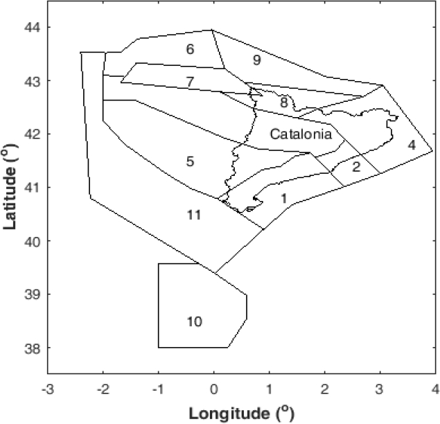
Table 1 Seismicity parameters of the seismic sources (Figure 1) in terms of macroseismic intensities [24]
| Seismic source |
Surface (km2) |
a | σ (a)* | β | σ (β)* |
h (km)* |
I min* | I max* |
I
max observed* |
|---|---|---|---|---|---|---|---|---|---|
| 1 | 14100 | 0.100 | 0.030 | 1.864 | 0.559 | 7 | V | VIII | VII |
| 2 | 4600 | 0.128 | 0.033 | 1.608 | 0.324 | 7 | V | IX | VIII |
| 4 | 16300 | 0.157 | 0.030 | 1.256 | 0.186 | 10 | V | X | IX |
| 5 | 23100 | 0.040 | 0.014 | 1.319 | 0.373 | 10 | V | IX | VIII |
| 6 | 8000 | 0.099 | 0.025 | 1.977 | 0.640 | 10 | V | VII | VI |
| 7 | 7200 | 0.957 | 0.090 | 1.420 | 0.116 | 15 | V | X | VIII |
| 8 | 7700 | 0.218 | 0.040 | 1.716 | 0.246 | 15 | V | IX | VIII |
| 9 | 9600 | 0.070 | 0.020 | 1.737 | 0.214 | 10 | V | VIII | VII |
| 10 | 19700 | 0.635 | 0.059 | 1.201 | 0.083 | 10 | V | XI | X |
| 11 | 40100 | 0.060 | 0.016 | 0.886 | 0.242 | 10 | V | IX | VIII |
* σ(α) is the standard deviation of α; σ(β) is the standard deviation of β; h is the depth in km; I min is the minimum epicentral intensity assigned to the seismic source; I max is the maximum epicentral intensity assigned to the seismic source; I max observed is the maximum epicentral intensity observed in the seismic source
At the same time, these seismicity parameters were applied in different studies to assess the seismic hazard of both Barcelona and Catalonia [5, 13, 14, 24]. Due to the wide validation of this seismicity parameters, we decided to use them also in the present study.
As a part of the procedure to compute seismic hazard in terms of exceedance rates of PGA, we applied relationships to convert macroseismic intensities (Table 1) to magnitudes. Particularly, we determined the seismicity parameters in terms of the magnitude Ms (surface wave magnitude), that is the type of magnitude required to use the GMPE of Ambraseys et al [6], which we chose for the present study.
The catalog of earthquakes for Barcelona is defined mainly in terms of macroseismic intensities. For this reason, the seismicity of the seismic sources (Figure 1 Fig. 1) was initially determined in terms of macroseismic intensities (Table 1). This seismicity was defined according to the truncated model of Gutenberg-Richter, that it is represented by Eq. (2):
where
In the section that follows, we mentioned the main criteria considered to compute the seismic parameters in terms of the magnitude Ms. However, it is convenient to highlight that if the seismicity parameters of the seismic sources are in terms of magnitudes, then Eq. (2) must be re-written to obtain Eq. (3):
where λ 0 is the exceedance rate of the magnitude M min , β is a parameter equivalent to the b-value of the Gutenberg-Richter relationship (Eq. (4)) for the seismic source (except that the parameter is given in terms of the natural logarithm), and M max is the maximum magnitude for the seismic source:
where N is the number of earthquakes with a magnitude greater or equal to M; a is the number of earthquakes with a magnitude greater than M min ; b is the slope of the line (called b-value).
Eq. (4) can be rewritten to obtain Eq. (5):
where α = a ln 10 and β = b ln 10. On the other hand, because usually the earthquakes are considered since a minimum magnitude (M min ), it is more practical to express the exceedance rate of the magnitude according to Eq. (6):
where
2.1.2 Ground Motion Prediction Equation
We choose the GMPE of Ambraseys et al [6] to assess the seismic hazard of Barcelona due mainly to the following reasons: a) this relationship was determined considering seismic records of 157 earthquakes in Europe and adjacent regions [6]; b) this GMPE was chosen to assess the seismic hazard of Barcelona during the Risk-UE project and in other recent studies [14]; c) this attenuation relationship has been chosen in diverse projects related to the assessment of the seismic hazard that involves to the region of Catalonia [13, 23], and the Iberian Peninsula [15].
The relationship of Ambraseys et al [6] is defined by Eq. (7):
where y is the acceleration in m/s2; M is equal to Ms. The value of r is computed according to Eq. (8):
d is the distance shorter to the projection to the failure plane in the surface of the earth in km, defined by Joyner and Boore [16];
Table 2 Values of the coefficients of Eq. (7) for the period T = 0 s
|
|
C 2 | h 0 | C 4 | C A | C S | σ |
|---|---|---|---|---|---|---|
| -1.48 | 0.266 | 3.5 | -0.922 | 0.117 | 0.124 | 0.25 |
Additionally, according to Ambraseys et al [6] the constants, S A and S S are equal to zero for a rock site. At the same time, Ambrasseys et al [6] defined that this GMPE can be applied when Ms is in the range between 4.0 and 7.5, and the distances from the seismic source are lower or equal to 200 km [6].
2.1.3 Data for Compute the 21 Different Curves of Seismic Hazard Associated to Each one of the 21 Cases Defined
The sensitivity analysis that we described in this document was oriented to determine the influence in the results of the seismic hazard of parameters of seismicity and parameters of the GMPE.
To perform the sensitivity analysis, we defined 21 different cases that were considered to compute seismic hazard. The difference is due to the data that we used to perform the PSHA. Each case was defined to contribute to identifying the influence of specific variables on the results of seismic hazard. Table 4 shows the main features that define to each one of the 21 cases considered in the present study.
Table 3 Summary of the features of each one of the 27 cases considered to compute the PSHA (from these 27 cases only 21 are different cases*)
| Parameters to be analyzed and cases | |||||||
|---|---|---|---|---|---|---|---|
| Relationship Magnitude vs Macroseismic Intensity to be considered | 1) Magnitude** | 2) β*** | 3) PGA from GMPE (Ambraseys et al [5])**** | ||||
| Values of magnitude | Case | Values of β | Case | Values of PGAs | Case | ||
| i) Ms-I 0 by López Casado et al [16] | a) mean - σ | 1ia | a) mean - σ | 2ia | a) mean - σ | 3ia | |
| b) mean | 1ib | b) mean | 2ib | b) mean | 3ib | ||
| c) mean + σ | 1ic | c) mean + σ | 2ic | c) mean + σ | 3ic | ||
| ii) Ms-I 0 by Gutdeutsch et al [11] | a) mean - σ | 1iia | a) mean - σ | 2iia | a) mean - σ | 3iia | |
| b) mean | 1iib | b) mean | 2iib | b) mean | 3iib | ||
| c) mean + σ | 1iic | c) mean + σ | 2iic | c) mean + σ | 3iic | ||
| iii) M L -I 0 by González [9] and Irizarry et al [13] | a) mean - σ | 1iiia | a) mean - σ | 2iiia | a) mean - σ | 3iiia | |
| b) mean | 1iiib | b) mean | 2iiib | b) mean | 3iiib | ||
| c) mean + σ | 1iiic | c) mean + σ | 2iiic | c) mean + σ | 3iiic | ||
* Notice that case 1ib = case 2ib = case 3ib; case 1iib = case 2iib = case 3iib; and case 1iiib = case 2iiib = case 3iiib.
** In these cases, the beta values are constant, and they are equal to the mean values.
*** In these cases, the magnitude values are constant, and they are equal to the mean values.
**** In these cases, both beta values and magnitude values are constant, and they are equal to the mean values.
Each case is identified by an ID defined by an Arabic number, a Roman number, and a letter (for instance in “1ia” the Arabic number allows to distinguish which parameter is analyzed between three options: 1) the magnitude; 2) the beta value; 3) the PGA value of the GMPE.
The Roman number allows to identify the relationship magnitude-macroseismic intensity, between three options: i) Ms-I 0 by López Casado et al, where I 0 is the epicentral distance; ii) Ms-I 0 by Gutdeutsch and; iii) M L -I 0 by Gonzalez and Irizarry et al, where M L means local magnitude. Finally, the letter in the ID allows to distinguish between the following options: a) mean values - σ; b) mean values and; c) mean values + σ.
For instance, according to Table 4 the curve of Case 1ia correspond to the curve where the following data were considered: 1 means that the analyzed parameter is the magnitude, therefore the beta values are constant values and they are equal to the mean values; i represents that the relationship Ms-I 0 by López Casado et al was applied; and the letter a means that the magnitude values were the mean values minus σ.
Similarly, in the curve of Case 2iib the number 2 means that the parameter analyzed is the beta value, therefore, the magnitude values are constant values; the number ii represents that the relationship Ms-I 0 by Gutdeutsch et al was applied, and finally, the letter b indicates that for the beta values the mean values were considered.
In the present study, we mainly analyzed the influence of three elements in the results of the curves of seismic hazard.
These elements are the following: A) the influence of the uncertainty on the magnitude values determined according to the particular relationship magnitude-macroseismic intensity chosen; B) the influence of the uncertainty associated with the assessment of the β values (Eq. (3)) and C) the influence of the uncertainty associated with the values of PGA determined according to the GMPE chosen. For this purpose, we compute the 21 seismic hazard curves summarized in Table 4.
2.2 Relationships of Magnitude versus Macroseismic Intensity
2.2.1 Common Data for Cases 1i, 1ii, and 1iii
In this section, we highlighted the common data used to compute the seismic hazard curves for the groups of cases 1i, 1ii, and 1iii.
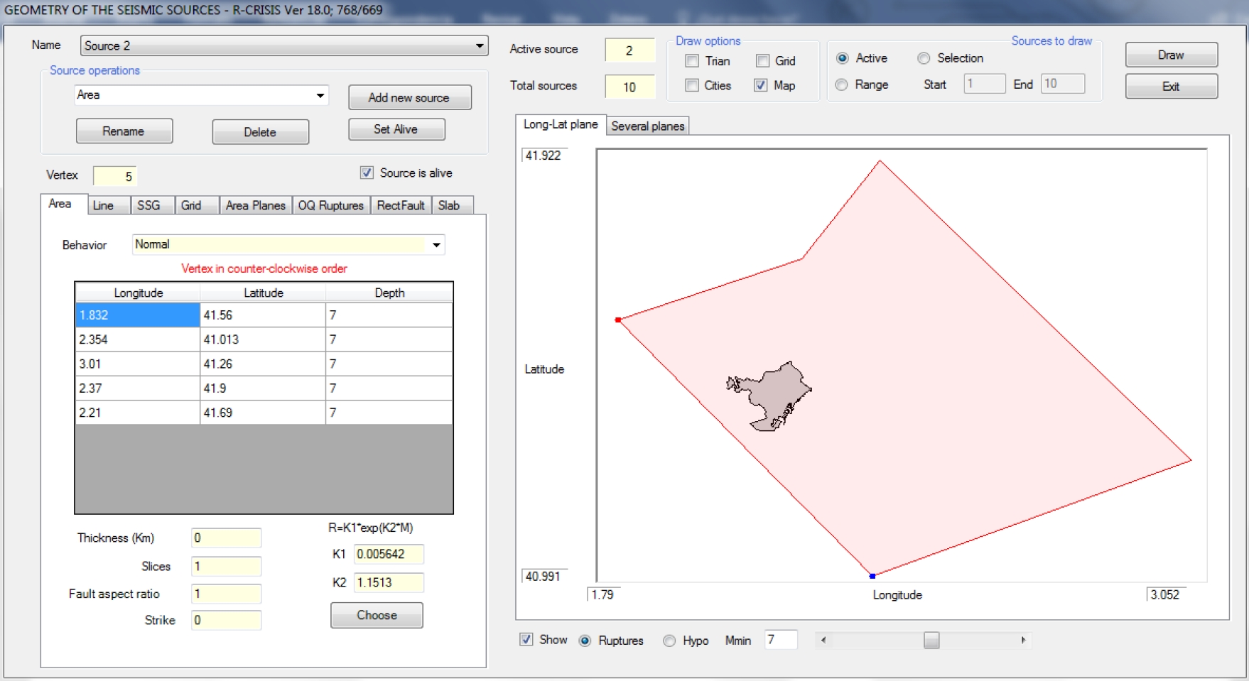
Particularly, for cases 1i, 1ii, and 1iii the common data is summarized in Table 5. On the other hand, Figure 2 shows the screen of R-CRISIS where the geometry of the seismic source number 2 (Figure 1) was defined. For each one of these groups of cases, we computed three seismic hazard curves, for instance, as is summarized in Table 4 for the case 1i we computed the curves 1ia,1ib, and 1ic.
2.2.2 Data for Cases 1ia, 1ib, and 1ic
Particularly, for the cases 1ia, 1ib, and 1ic the seismicity for each seismic source was defined with the data of Table 2 and Table 3 and according to Table 4. The values of magnitude in Table 3 were mainly determined with the data of Table 4 and the relationship summarized in Eq. (9):
where I 0 is the epicentral intensity (MSK), 0.7 is the standard deviation, P is equal to 0 to determine mean values (percentile 50), or equal to 1 to determine the values of the percentile 84. Additionally, to assess the values of the percentile 16 we considered P equal to -1, that correspond to the mean values minus a standard deviation. Eq. (9) is mainly valid for the range II ≤ I 0 ≤ X, and 1.6 ≤ Ms ≤ 7.0 [17].
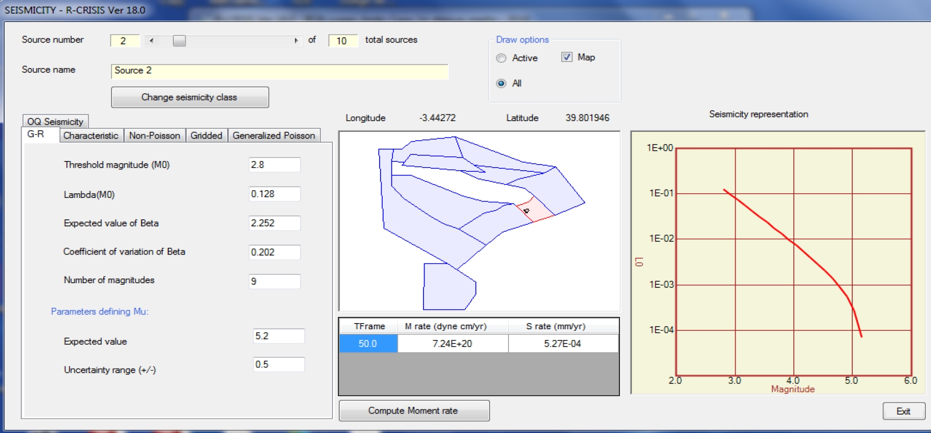
Figure 3 shows the screen of R-CRISIS where we assigned the seismicity parameters for the case 1ib. If the purpose of the present assessment would have been developing a PSHA to obtain a representative seismic hazard curve, then the curve of the case 1ib could have been that representative curve. However, we also computed the cases 1ia and 1ic as a part of the sensitivity analysis in the present study.
Particularly, for the case 1ia, we used as data the mean values minus a standard deviation (Table 3) as if they were the mean values that are required by R-CRISIS to compute the seismic hazard. Similarly, for the case 1ic, we used as data the mean values plus a standard deviation (Table 3) as if they were the mean values that are required by R-CRISIS to determine the seismic hazard.
2.2.3 Data for Cases 1iia, 1iib, and 1iic
The unique difference between the cases 1iia, 1iib, and 1iic (Table 4) and the cases 1ia, 1ib, and 1ic is the relationship magnitude-macroseismic intensity used. We applied the relationship defined by Gutdeutsch et al [12] for the cases 1iia, 1iib, and 1iic (Table 4). This relationship was defined for the South of Europe and it is represented by Eq. (10):
where I 0 is the epicentral distance. Eq. (10) has a standard deviation of ± 0.412 and it is valid for 4 ≤ Ms ≤ 7 and depths lower than 50 km [12].
Table 8 and Table 9 shows the parameters for the seismic sources for the cases 1iia, 1iib, and 1iic. We computed these parameters according to the data of Table 4 and Eq. (10).
Table 6 Seismicity parameters (Poisson model) for the seismic sources whose geometry is shown in Figure 1 and for cases 1ia, 1ib, and 1ic
| Seismic source | h (km) | λ(M min ) | β | Coefficient of variation β |
|---|---|---|---|---|
| 1 | 7 | 0.100 | 2.811 | 0.300 |
| 2 | 7 | 0.128 | 2.252 | 0.202 |
| 4 | 10 | 0.157 | 1.642 | 0.148 |
| 5 | 10 | 0.040 | 1.847 | 0.283 |
| 6 | 10 | 0.099 | 3.230 | 0.324 |
| 7 | 15 | 0.957 | 1.856 | 0.082 |
| 8 | 15 | 0.218 | 2.403 | 0.143 |
| 9 | 10 | 0.070 | 2.620 | 0.123 |
| 10 | 10 | 0.635 | 1.472 | 0.069 |
| 11 | 10 | 0.060 | 1.241 | 0.273 |
Table 7 Seismicity values for cases 1ia, 1ib, and 1ic
| Seismic Source |
Mean values- σ | Mean values | Mean values + σ | ||||||
|---|---|---|---|---|---|---|---|---|---|
| M min * | M max | M min * | M max | M min * | M max | ||||
| E(M max )* | (Upper limit of M max -lower limit of M max )/2 | E(M max )* | (Upper limit of M max -lower limit of M max )/2 | E(M max )* | (Upper limit of M max -lower limit of M max )/2 | ||||
| 1 | 2.1 | 3.7 | 0.4 | 2.8 | 4.4 | 0.4 | 3.5 | 5.1 | 0.4 |
| 2 | 2.1 | 4.5 | 0.5 | 2.8 | 5.2 | 0.5 | 3.5 | 5.9 | 0.5 |
| 4 | 2.1 | 5.4 | 0.5 | 2.8 | 6.1 | 0.5 | 3.5 | 6.8 | 0.5 |
| 5 | 2.1 | 4.5 | 0.5 | 2.8 | 5.2 | 0.5 | 3.5 | 5.9 | 0.5 |
| 6 | 2.1 | 2.8 | 0.5 | 2.8 | 3.5 | 0.5 | 3.5 | 4.2 | 0.5 |
| 7 | 2.1 | 5.0 | 0.9 | 2.8 | 5.7 | 0.9 | 3.5 | 6.4 | 0.9 |
| 8 | 2.1 | 4.5 | 0.5 | 2.8 | 5.2 | 0.5 | 3.5 | 5.9 | 0.5 |
| 9 | 2.1 | 3.7 | 0.4 | 2.8 | 4.4 | 0.4 | 3.5 | 5.1 | 0.4 |
| 10 | 2.1 | 6.4 | 0.6 | 2.8 | 7.1 | 0.6 | 3.5 | 7.8 | 0.6 |
| 11 | 2.1 | 4.5 | 0.5 | 2.8 | 5.2 | 0.5 | 3.5 | 5.9 | 0.5 |
* M min is the minimum magnitude considered in the i-esim seismic source; E(M max ) is the value of the maximum magnitude expected in the i-esim seismic source
Table 8 Seismicity values for cases 1iia, 1iib, and 1iic
| Seismic source |
Mean values - σ | Mean values | Mean values + σ | ||||||
|---|---|---|---|---|---|---|---|---|---|
| M min * | M max | M min * | M max | M min * | M max | ||||
| E(M max )* | (Upper limit of M max -lower limit of M max )/2 | E(M max )* | (Upper limit of M max -lower limit of M max )/2 | E(M max )* | (Upper limit of M max -lower limit of M max )/2 | ||||
| 1 | 3.6 | 5.0 | 0.3 | 4.0 | 5.4 | 0.3 | 4.4 | 5.8 | 0.3 |
| 2 | 3.6 | 5.5 | 0.3 | 4.0 | 5.9 | 0.3 | 4.4 | 6.4 | 0.2 |
| 4 | 3.6 | 6.1 | 0.2 | 4.0 | 6.5 | 0.3 | 4.4 | 6.9 | 0.3 |
| 5 | 3.6 | 5.5 | 0.3 | 4.0 | 5.9 | 0.3 | 4.4 | 6.4 | 0.2 |
| 6 | 3.6 | 4.4 | 0.3 | 4.0 | 4.8 | 0.3 | 4.4 | 5.3 | 0.2 |
| 7 | 3.6 | 5.8 | 0.5 | 4.0 | 6.2 | 0.6 | 4.4 | 6.6 | 0.6 |
| 8 | 3.6 | 5.5 | 0.3 | 4.0 | 5.9 | 0.3 | 4.4 | 6.3 | 0.3 |
| 9 | 3.6 | 5.0 | 0.3 | 4.0 | 5.4 | 0.3 | 4.4 | 5.8 | 0.3 |
| 10 | 3.6 | 6.6 | 0.3 | 4.0 | 7.0 | 0.3 | 4.4 | 7.4 | 0.3 |
| 11 | 3.6 | 5.5 | 0.3 | 4.0 | 5.9 | 0.3 | 4.4 | 6.4 | 0.2 |
* M min is the minimum magnitude considered in the i-esim seismic source; E(M max ) is the value of the maximum magnitude expected in the i-esim seismic source
Table 9 Seismicity parameters for seismic sources for cases 1iia, 1iib, and 1iic
| Seismic source |
h (km) | λ(M min ) | β | Coef. of variation β |
|---|---|---|---|---|
| 1 | 7 | 0.100 | 3.389 | 0.300 |
| 2 | 7 | 0.128 | 2.924 | 0.202 |
| 4 | 10 | 0.157 | 2.284 | 0.148 |
| 5 | 10 | 0.040 | 2.398 | 0.283 |
| 6 | 10 | 0.099 | 3.595 | 0.324 |
| 7 | 15 | 0.957 | 2.582 | 0.082 |
| 8 | 15 | 0.218 | 3.120 | 0.143 |
| 9 | 10 | 0.070 | 3.158 | 0.123 |
| 10 | 10 | 0.635 | 2.184 | 0.069 |
| 11 | 10 | 0.060 | 1.611 | 0.273 |
2.2.4 Data for Cases 1iiia, 1iiib, and 1iiic
The main difference between the cases 1iiia, 1iiib, and 1iiic (Table 2), and the previous groups of cases 1i and 1ii is again the relationship magnitude-macroseismic intensity used. In the group of the cases 1iii was necessary to apply two relationships, the first one to convert macroseismic intensities in values of M L (local magnitude), and the second one to convert values of M L in values of M S . The relationships to obtain values of M L were determined for Catalonia by Gonzalez [10] and Irizarry et al [14]. These relationships are summarized in Eq. (11, 12, 13).
The seismic parameters determined according to the data in Table 1 are summarized in Table 10 Additionally, we applied the relationship of Gutdeutsch et al [12] represented by Eq. (14) to obtain the seismic parameters for the seismic sources in terms of M S Table 11:
Table 10 Seismicity parameters in terms of M S for cases 1iiia, 1iiib, and 1iiic
| Seismic Source |
h (km) | M min | λ(M min ) | β | M max |
|---|---|---|---|---|---|
| 1 | 7 | 3.8 | 0.100 | 3.585 | 5.4 |
| 2 | 7 | 3.8 | 0.128 | 3.092 | 5.9 |
| 4 | 10 | 4.1 | 0.157 | 2.415 | 6.7 |
| 5 | 10 | 4.1 | 0.040 | 2.537 | 6.2 |
| 6 | 10 | 4.1 | 0.099 | 3.802 | 5.1 |
| 7 | 15 | 4.4 | 0.957 | 2.731 | 7.0 |
| 8 | 15 | 4.4 | 0.218 | 3.300 | 6.5 |
| 9 | 10 | 4.1 | 0.070 | 3.340 | 5.7 |
| 10 | 10 | 4.1 | 0.635 | 2.310 | 7.2 |
| 11 | 10 | 4.1 | 0.060 | 1.704 | 6.2 |
Table 11 Additional seismicity parameters in terms of Ms for cases 1iiia, 1iiib, and 1iic
| Seismic source |
h (km) | λ(M min ) | β | Coef. variation β |
|---|---|---|---|---|
| 1 | 7 | 0.100 | 3.201 | 0.300 |
| 2 | 7 | 0.128 | 2.761 | 0.202 |
| 4 | 10 | 0.157 | 2.157 | 0.148 |
| 5 | 10 | 0.040 | 2.265 | 0.283 |
| 6 | 10 | 0.099 | 3.395 | 0.324 |
| 7 | 15 | 0.957 | 2.439 | 0.082 |
| 8 | 15 | 0.218 | 2.950 | 0.143 |
| 9 | 10 | 0.070 | 2.983 | 0.123 |
| 10 | 10 | 0.635 | 2.063 | 0.069 |
| 11 | 10 | 0.060 | 1.522 | 0.273 |
where h is the depth in km.
Eq. (14) has a standard deviation of ± 0.163.
2.2.5 Common Data for Cases 2ia, 2ib, and 2ic
As it was mentioned previously, another parameter that we considered for the sensitivity analysis was the parameter β.
For this purpose, we computed curves of seismic hazard considering the different values of β that can be obtained according to the three cases of relationships magnitude-macroseismic intensities considered in the present study. Table 12 shows the common data for cases 2i, 2ii, and 2iii.
2.2.6 Data for Cases 2ia, 2ib, and 2ic
Table 14 and Table 15 shows the seismicity data for each seismic source that we used for the cases 2ia, 2ib, and 2ic. Particularly, for the three cases, we used all the data of Table 14. However, for the case 2ia, we used only the mean values of β minus σ 0Table 15 as if they were the mean values that are required by R-CRISIS to compute the seismic hazard. In the same way, for the case 2ib we used only the mean values of β (Table 15). Additionally, for the case 2ic, we used only the mean values of β plus σ (Table 15).
Table 13 Seismicity values of the seismic sources for cases 1iiia, 1iiib, and 1iiic
| Seismic source |
Mean values - σ | Mean values | Mean values + σ | ||||||
|---|---|---|---|---|---|---|---|---|---|
| M min | M max | M max | M max | ||||||
| E(M max ) | (Upper limit of M max -lower limit of M max )/2 | M min | E(M max ) | (Upper limit of M max -lower limit of M max )/2 | M min | E(M max ) | (Upper limit of M max -lower limit of M max )/2 | ||
| 1 | 3.4 | 4.8 | 0.3 | 3.5 | 5.0 | 0.3 | 3.7 | 5.1 | 0.3 |
| 2 | 3.4 | 5.4 | 0.3 | 3.5 | 5.6 | 0.2 | 3.7 | 5.7 | 0.3 |
| 4 | 3.7 | 6.3 | 0.3 | 3.8 | 6.5 | 0.3 | 4.0 | 6.6 | 0.3 |
| 5 | 3.7 | 5.7 | 0.3 | 3.8 | 5.9 | 0.3 | 4.0 | 6.0 | 0.3 |
| 6 | 3.7 | 4.6 | 0.3 | 3.8 | 4.7 | 0.3 | 4.0 | 4.9 | 0.3 |
| 7 | 4.0 | 6.4 | 0.5 | 4.2 | 6.5 | 0.6 | 4.3 | 6.7 | 0.6 |
| 8 | 4.0 | 6.1 | 0.3 | 4.2 | 6.2 | 0.3 | 4.3 | 6.4 | 0.3 |
| 9 | 3.7 | 5.1 | 0.3 | 3.8 | 5.3 | 0.3 | 4.0 | 5.5 | 0.3 |
| 10 | 3.7 | 6.9 | 0.3 | 3.8 | 7.1 | 0.2 | 4.0 | 7.2 | 0.3 |
| 11 | 3.7 | 5.7 | 0.3 | 3.8 | 5.9 | 0.3 | 4.0 | 6.0 | 0.3 |
Table 14 Seismic parameters of the seismic sources for cases 2ia, 2ib, and 2ic
| Seismic source |
h (km) | M min mean | λ(M min ) | Coef. variation β | M max mean | (Upper limit of M max -lower limit of M max )/2 |
|---|---|---|---|---|---|---|
| 1 | 7 | 2.8 | 0.100 | 0.300 | 4.4 | 0.4 |
| 2 | 7 | 2.8 | 0.128 | 0.202 | 5.2 | 0.5 |
| 4 | 10 | 2.8 | 0.157 | 0.148 | 6.1 | 0.5 |
| 5 | 10 | 2.8 | 0.040 | 0.283 | 5.2 | 0.5 |
| 6 | 10 | 2.8 | 0.099 | 0.324 | 3.5 | 0.5 |
| 7 | 15 | 2.8 | 0.957 | 0.082 | 5.7 | 0.9 |
| 8 | 15 | 2.8 | 0.218 | 0.143 | 5.2 | 0.5 |
| 9 | 10 | 2.8 | 0.070 | 0.123 | 4.4 | 0.4 |
| 10 | 10 | 2.8 | 0.635 | 0.069 | 7.1 | 0.6 |
| 11 | 10 | 2.8 | 0.060 | 0.273 | 5.2 | 0.5 |
2.2.7 Data for cases 2iia, 2iib, and 2iic
Particularly, for the cases 2iia, 2iib, and 2iic the seismicity for each seismic source is defined with data of Table 16 and Table 17 For instance, for the case 2iia, we used all the data of Table 16 and only the mean values of β minus σ (Table 17).
Table 16 Seismicity parameters of the seismic sources for cases 2iia, 2iib, and 2iic
| Seismic source |
h (km) | M min mean | λ(M min ) | Coef. variation β | M max mean | (Upper limit of M max -lower limit of M max )/2 |
|---|---|---|---|---|---|---|
| 1 | 7 | 4 | 0.100 | 0.3 | 5.4 | 0.3 |
| 2 | 7 | 4 | 0.128 | 0.202 | 5.9 | 0.3 |
| 4 | 10 | 4 | 0.157 | 0.148 | 6.5 | 0.3 |
| 5 | 10 | 4 | 0.040 | 0.283 | 5.9 | 0.3 |
| 6 | 10 | 4 | 0.099 | 0.324 | 4.8 | 0.3 |
| 7 | 15 | 4 | 0.957 | 0.082 | 6.2 | 0.6 |
| 8 | 15 | 4 | 0.218 | 0.143 | 5.9 | 0.3 |
| 9 | 10 | 4 | 0.070 | 0.123 | 5.4 | 0.3 |
| 10 | 10 | 4 | 0.635 | 0.069 | 7.0 | 0.3 |
| 11 | 10 | 4 | 0.060 | 0.273 | 5.9 | 0.3 |
Table 17 Values of beta for the cases 2iia, 2iib, and 2iic
| Seismic source |
β | ||
|---|---|---|---|
| mean - σ | mean | mean + σ |
|
| 1 | 2.373 | 3.389 | 4.405 |
| 2 | 2.335 | 2.924 | 3.513 |
| 4 | 1.945 | 2.284 | 2.622 |
| 5 | 1.720 | 2.398 | 3.076 |
| 6 | 2.431 | 3.595 | 4.758 |
| 7 | 2.371 | 2.582 | 2.793 |
| 8 | 2.673 | 3.120 | 3.567 |
| 9 | 2.769 | 3.158 | 3.547 |
| 10 | 2.033 | 2.184 | 2.335 |
| 11 | 1.171 | 1.611 | 2.051 |
Similarly, for the case 2iib, we used all the data of Table 16 and only the mean values of β (Table 17) Moreover, for the case 2iic, we used all the data of Table 16 and only the mean values of β plus σ (Table 17).
2.2.8 Data for Cases 2iiia, 2iiib, and 2iiic
Specifically, for the cases 2iiia, 2iiib, and 2iiic the seismicity for each seismic source is defined with the data of Table 18 and Table 19. Particularly, for the three cases, we used all the data of Table 18. However, for the case 2iiia, we used only the mean values of β minus σ (Table 19). Similarly, for the case 2iiib, we used only the mean values of β (Table 19). Furthermore, for the case 2iiic, we used the mean values of β plus σ (Table 19).
Table 18 Seismicity parameters of the seismic sources for the cases 2iiia, 2iiib, and 2iiic
| Seismic source |
h (km) | M min mean | λ(M min ) | Coef. variation β | M max mean | (Upper limit of Mmax -lower limit of Mmax)/2 |
|---|---|---|---|---|---|---|
| 1 | 7 | 3.5 | 0.100 | 0.3 | 5.0 | 0.3 |
| 2 | 7 | 3.5 | 0.128 | 0.202 | 5.6 | 0.2 |
| 4 | 10 | 3.9 | 0.157 | 0.148 | 6.5 | 0.3 |
| 5 | 10 | 3.9 | 0.040 | 0.283 | 5.9 | 0.3 |
| 6 | 10 | 3.9 | 0.099 | 0.324 | 4.7 | 0.3 |
| 7 | 15 | 4.2 | 0.957 | 0.082 | 6.5 | 0.6 |
| 8 | 15 | 4.2 | 0.218 | 0.143 | 6.2 | 0.3 |
| 9 | 10 | 3.9 | 0.070 | 0.123 | 5.3 | 0.3 |
| 10 | 10 | 3.9 | 0.635 | 0.069 | 7.1 | 0.2 |
| 11 | 10 | 3.9 | 0.060 | 0.273 | 5.9 | 0.3 |
Table 19 Values of beta for the cases 2iiia, 2iiib, and 2iiic
| Seismic source |
β | ||
|---|---|---|---|
| mean - σ | mean | mean + σ |
|
| 1 | 2.241 | 3.201 | 4.161 |
| 2 | 2.205 | 2.761 | 3.318 |
| 4 | 1.838 | 2.157 | 2.476 |
| 5 | 1.625 | 2.265 | 2.906 |
| 6 | 2.296 | 3.395 | 4.494 |
| 7 | 2.239 | 2.439 | 2.638 |
| 8 | 2.524 | 2.950 | 3.369 |
| 9 | 2.615 | 2.983 | 3.350 |
| 10 | 1.920 | 2.063 | 2.205 |
| 11 | 1.106 | 1.522 | 1.937 |
2.2.9 Common Data for Cases 3ia, 3ib, and 3ic
In the group of cases 3, the sensitivity analysis consisted in to assess the seismic hazard with the emphasis in the uncertainty in the values of PGA, according to the GMPE of Ambrasseys et al [6] chosen in the present study. Table 20 shows the common data for cases 3i, 3ii, and 3iii.
Table 20 Common data for the cases 3i, 3ii, and 3iii
| Concept | Data | |
|---|---|---|
| Site of computation | Longitude: 2.195 degrees | Latitude: 41.42 degrees |
| Geometry of the seismic sources | Figure 1 | |
2.2.10 Data for Cases 3ia, 3ib, and 3ic
Particularly, for the cases 3ia, 3ib, and 3ic the seismicity for each seismic source is defined with the data of Table 14 and the mean values of β of Table 15. Additionally, for the case 3ia, we used only the mean values of PGA minus σ of the GMPE (Eq. (7)) as if they were the mean values that are required by R-CRISIS to compute the seismic hazard. For the case 3ib, we used only the mean values of PGA of the GMPE. In the same way, for the case 3ic, we used only the mean values of PGA plus σ of the GMPE.
2.2.11 Data for Cases 3iia, 3iib, and 3iic
Specifically, for the cases 3iia, 3iib, and 3iic the seismicity for each seismic source is defined with the data of Table 16 and the mean values of β of Table 17. Moreover, for the case 3iia, we used only the mean values of PGA minus σ of the GMPE (Eq. (7)). For the case 3iib, we used only the mean values of PGA of the GMPE. Likewise, for the case 3iic, we just used the mean values of PGA plus σ of the GMPE.
2.2.12 Data for Cases 3iiia, 3iiib, and 3iiic
For the cases 3iiia, 3iiib, and 3iiic the seismicity for each seismic source is defined with the data of Table 18 and the mean values of β of Table 19. Furthermore, for the case 3iiia, we used only the mean values of PGA minus σ of the GMPE. For the case 3iiib, we just used the mean values of PGA of the GMPE. Similarly, for the case 3iiic, we used only the mean values of PGA plus σ of the GMPE.
3. Results of the Sensitivity Analysis for the PSHA of Barcelona
3.1 Performing PSHA with R-CRISIS
As it was mentioned previously, we used the code R-CRISIS to perform PSHA. This code was published at the end of 2017. R-CRISIS is a freeware and standalone code that in the present study was executed in a Laptop with a processor Intel ® Core™ i5-3210M CPU @ 2.50GHz 2.50GHz, and operative system Windows 7 Professional. We made an input file for each case of Table 4. At the same time, we generated a seismic hazard curve for each case. We show in the next section the seismic hazard curves that we computed with R-CRISIS.
Moreover, it is possible to mention that at the beginning of the present study we used the software CRISIS2015 [2, 20], however, at the end of 2017 an updated version of CRISIS2015 called R-CRISIS [21] was published. Therefore, we started to use the new version of CRISIS as soon as it was available. About the use of R-CRISIS, we can mention that we used the input files generated with CRISIS2015 to compute seismic hazard with R-CRISIS. Therefore, R-CRISIS can read without difficulties data files generated in CRISIS2015.
3.2 Analysis of the Main Results of PSHA for the Different Cases
We obtained graphs for each group of seismic hazard curves to analyze the results. For instance, we can observe the three curves of the cases 1i in the same graph (Figure 4). In the present section, we show the seismic hazard curves for the 27 cases of Table 4. At the same time, we highlighted some particularities between the seismic hazard curves obtained.
In the seismic hazard curves of Figure 4, we can identify the size of the influence in the results of seismic hazard of the uncertainty associated to the relation magnitude-macroseismic intensity of López Casado et al [17]. This last affirmation is because the differences between the three curves are essentially attributable to the different levels of uncertainty considered for the values of magnitude (M s ) determined through the relationship of López Casado et al [17].
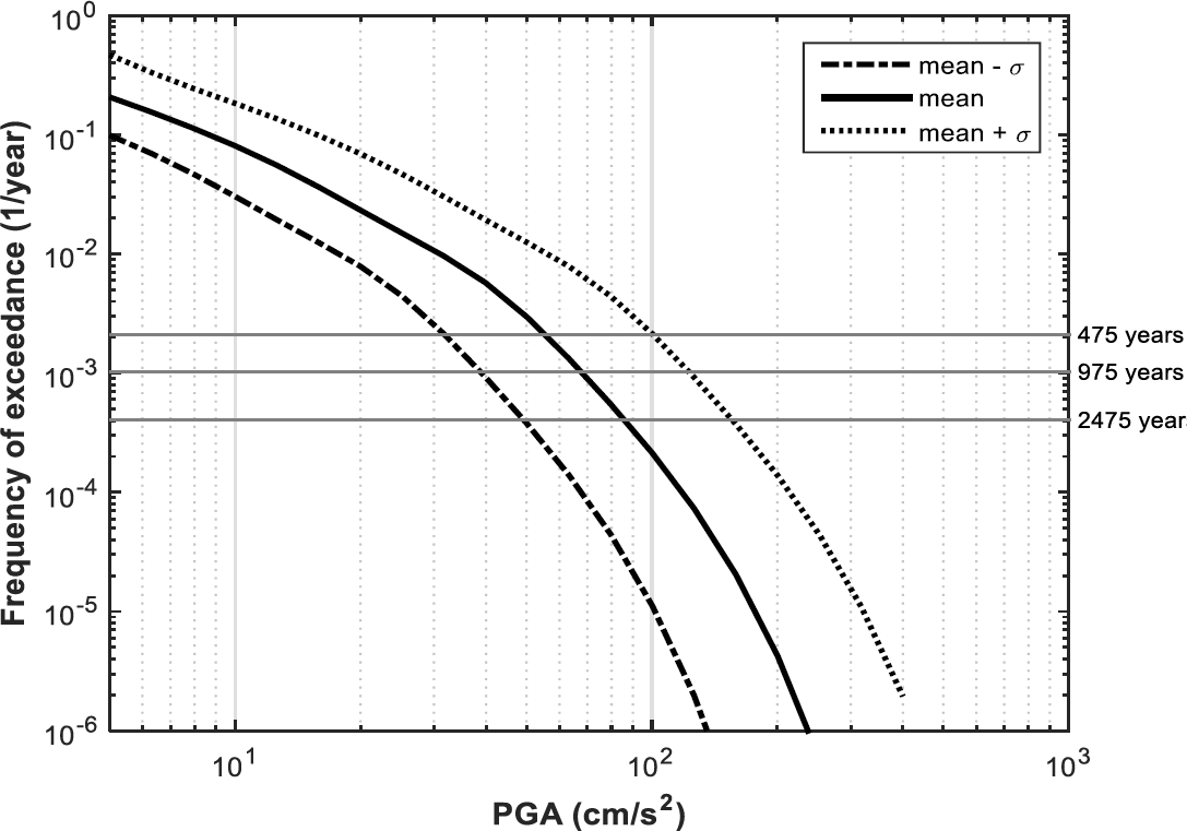
3.2.1 Seismic Hazard Curves of Barcelona for Cases 1ia, 1ib, and 1ic
Figure 4 shows the seismic hazard curves that we computed for the cases 1ia, 1ib, and 1ic. The difference between these curves is basically attributable to the different levels of uncertainty considered for the values of magnitude according to the relation magnitude-macroseismic intensity represented by Eq. (3).
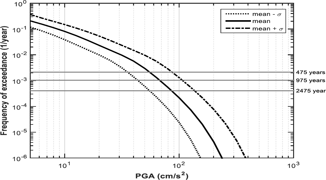
Particularly, according to the results of Figure 4 the value of PGA in Barcelona (for a rock site and for a return period of 475 years) ranges from 35 cm/s2 (case 1ia) to 88 cm/s2 (case 1ic), with a mean value of 55 cm/s2 (case 1ib). These means, for instance, that the seismic hazard computed in case 1ic (for a return period of 475 years) is 60% greater than the value computed in case 1ib.
3.2.2 Seismic Hazard Curves of Barcelona for Cases 1iia, 1iib, and 1iic
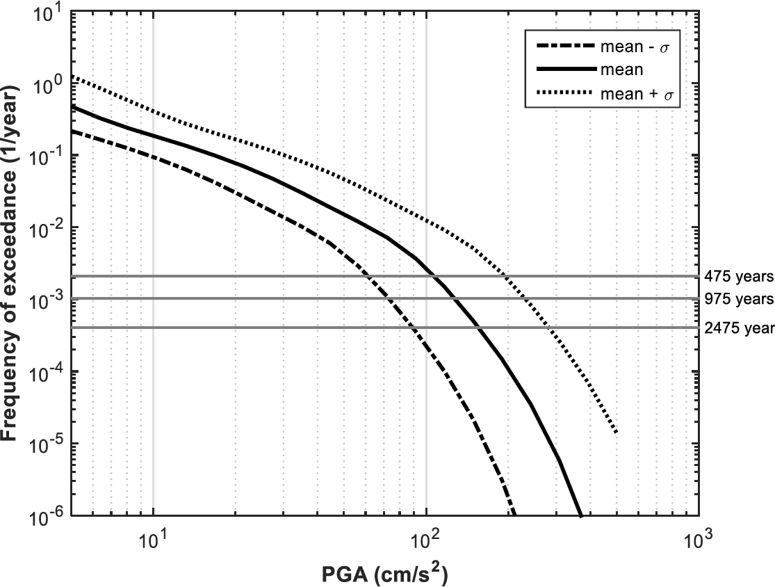
The seismic hazard curves of Figure 5 correspond to the cases 1iia, 1iib, and 1iic. In these cases, the differences between the three curves are fundamentally attributable to the different levels of uncertainty considered for the values of magnitude according to the relation magnitude-macroseismic intensity represented by Eq. (10).

It is possible to notice that according to Figure 5 the value of PGA in Barcelona (for a rock site and for a return period of 475 years) ranges from 82 cm/s2 (case 1iia) to 140 cm/s2 (1iic), with a mean value of 106 cm/s2 (1iib). These results also mean that the seismic hazard computed in case 1iic (for a return period of 475 years) is 1.3 times greater than the value computed for case 1iib.
3.2.3 Seismic Hazard Curves of Barcelona for Cases 1iiia, 1iiib, and 1iiic
In the same way as the previous cases, Figure 6 shows the seismic hazard curves for cases 1iiia, 1iiib, and 1iiic. In these cases, the differences between the three curves are also essentially attributable to different levels of uncertainty considered for the values of magnitude according to the relation magnitude-macroseismic intensity represented by Eqs. (1, 2, 3, 4).
According to Figure 6 the value of PGA in Barcelona (for a rock site and for a return period of 475 years) ranges from 74 cm/s2 (case 1iiia) to 89 cm/s2 (case 1iiic) with a mean value of 79 cm/s2 (case 1iiib). These also means that the seismic hazard computed in case 1iiic for a return period of 475 years is 13% greater than the value for case 1iiib.
Table 21 shows a summary of the results of PGA for cases 1i, 1ii, and 1iii for a return period of 475 years according to the seismic hazard curves of Figure 4, Figure 5 and Figure 6.
3.2.4 Seismic Hazard Curves of Barcelona for Cases 2ia, 2ib, and 2ic
Figure 7 shows the seismic hazard curves for the cases 2ia, 2ib, and 2ic. In these cases, the differences between the three curves are essentially attributable to the uncertainty associated with the β parameter.
According to the results for cases 2i (Figure 7) the value of PGA in Barcelona (for a rock site and for a return period of 475 years) ranges from 52 cm/s2 (2ia) to 61 cm/s2 (2ic), with a mean value of 55 cm/s2 (2ib). These results also mean that an increment in one standard deviation of the β values generates an increment of 11% in the results of seismic hazard, for a return period of 475 years.
3.2.5 Seismic Hazard Curves of Barcelona for Cases 2iia, 2iib, and 2iic
In the same way as the group of cases 2i, Figure 8 shows the seismic hazard curves for the cases 2iia, 2iib, and 2iic. In these cases, the differences between the curves are also basically attributable to the uncertainty associated with the β parameter. According to the results (Figure 8), the value of PGA in Barcelona (for a rock site and for a return period of 475 years) ranges from 100 cm/s2 (case 2iia) to 115 cm/s2 (2iic), with a mean value of 106 cm/s2 (2iib). In these cases, the difference between the results of PGA computed for a return period of 475 years is about 6.0% between cases 2iia and 2iib, and about 8.5% between cases 2iib and 2iic.
3.2.6 Seismic Hazard Curves of Barcelona for Cases 2iiia, 2iiib, and 2iiic
Finally, for the group of cases 2, we determined the Figure 9 which shows the seismic hazard curves for cases 2iiia, 2iiib, and 2iiic. In these cases, the differences between the curves are also fundamentally attributable to the uncertainty associated with the β parameter. According to the results (Figure 8) for these cases, the value of PGA in Barcelona (for a rock site and for a return period of 475 years) ranges from 75 cm/s2 (2iiia) to 90 cm/s2 (2iiic), with a mean value of 79 cm/s2 (2iiib). These results also mean that an increment in one standard deviation of the β values generates an increment of 14% in the results of seismic hazard, for a return period of 475 years.
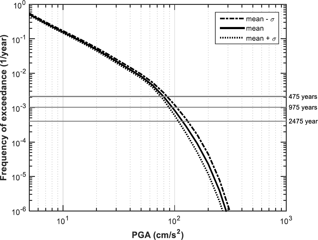
Table 22 shows a summary of the results of PGA for cases 2i, 2ii, and 2iii for a return period of 475 years, according to the seismic hazard curves of Figure 7, Figure 8 and Figure 9.
3.2.7 Seismic Hazard Curves of Barcelona for Cases 3ia, 3ib, and 3ic
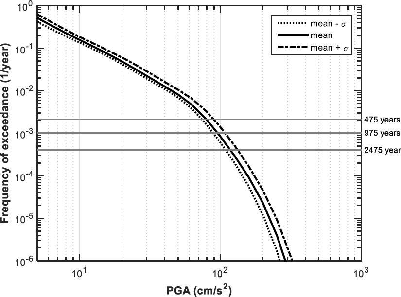
The last group of cases that we analyzed was the group 3. Figure 10 shows the seismic hazard curves for cases 3ia, 3ib, and 3ic. In these cases, the differences between the curves are essentially attributable to the uncertainty associated with the values of PGA according to the GMPE chosen in the present study. According to the results (Figure 10 ) for these cases, the value of PGA in Barcelona (for a rock site and for a return period of 475 years) ranges from 32 cm/s2 (3ia) to 100 cm/s2 (3ic), with a mean value of 55 cm/s2 (3ib). It is possible to observe that the difference between the three cases is important. For instance, the value of PGA for a return period of 475 years for the case 3ic is 82% greater than the result for the case 3ib.
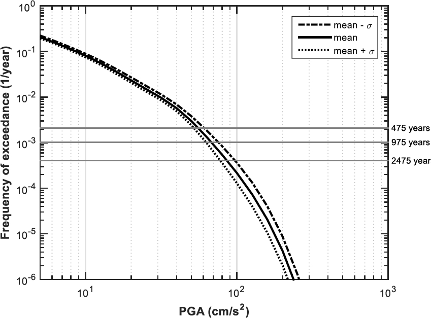
3.2.8 Seismic Hazard Curves of Barcelona for Cases 3iia, 3iib, and 3iic
Figure 11 shows the three seismic hazard curves for cases 3iia, 3iib, and 3iic. In these cases, the differences between the three curves are also fundamentally attributable to the uncertainty associated with the values of PGA according to the GMPE chosen in the present study.
According to the results of Figure 11 the value of PGA in Barcelona (for a rock site and for a return period of 475 years) ranges from 61 cm/s2 (3iia) to 192 cm/s2 (3iic) with a mean value of 106 cm/s2 (3iib). It is possible to observe that there are important differences between the results for these cases. For instance, the value of PGA for a return period of 475 years for the case 3iic is 81% greater than the value of PGA for the case 3iib.
3.2.9 Seismic Hazard Curves of Barcelona for Cases 3iiia, 3iiib, and 3iiic
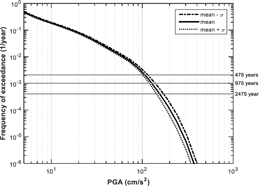
Finally, Figure 12 shows the seismic hazard curves for cases 3iiia, 3iiib, and 3iiic. In these cases, the differences between the three curves are also basically attributable to the uncertainty associated with the values of PGA according to the GMPE chosen in the present study. According to the results (Figure 12) for these cases, the value of PGA in Barcelona (for a rock site and for a return period of 475 years) ranges from 46 cm/s2 (3iiia) to 144 cm/s2 (3iiic) with a mean value of 79 cm/s2 (3iiib).
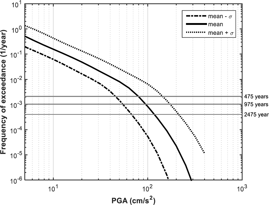
Fig. 12. Seismic hazard curves of Barcelona for cases 3iiia (mean - σ), 3iiib (mean), and 3iiic (mean + σ)
Table 23 shows a summary of the results of PGA for cases 3i, 3ii, and 3iii for a return period of 475 years according to the seismic hazard curves of Figure 10, Figure 11 and Figure 12.
4 Conclusion
According to the results of the group of cases 1i, 1ii, and 1iii it is possible to conclude that in general, the relation magnitude-macroseismic intensity (chosen to determine part of the data required to compute seismic hazard) have a significant influence in the results of seismic hazard of Barcelona. The size of the influence is mainly related with the value of the standard deviation associated with the relation magnitude-macroseismic intensity, that was chosen to obtain the data required to perform the PSHA.
Similarly, according to the results of the cases of the groups 2i, 2ii, and 2iii, it is possible to conclude that the uncertainty related to the β parameter, has a moderate influence in the results of seismic hazard of Barcelona. This conclusion is due to the fact, that the maximum increment in the values of PGA between two adjacent curves of seismic hazard for a return period of 475 years was of 14% between the cases 2iiib and 2iiic.
According to the results of the cases of the groups 3i, 3ii and 3iii, it is possible to conclude that the uncertainty related to the GMPE has a significant influence in the results of seismic hazard of Barcelona. This conclusion is based on the fact, that the maximum increment in the values of PGA between two adjacent curves of seismic hazard for a return period of 475 years was of 82% between the cases 3iiib and 3iiic.
Additionally, it is possible to conclude that the major influence in the determination of the results of seismic hazard for Barcelona was related to the values of PGA determined according to the GMPE chosen. However, the relationship magnitude-macroseismic intensity also have an important influence in the results of seismic hazard. Being the value of the parameter Beta, the variable that has the lower influence in the results of seismic hazard for Barcelona according to the data and procedures that we applied in the present study.
The previous results allow concluding that the election of the GMPE and the relationship magnitude-macroseismic intensities have a fundamental influence on the results of seismic hazard for Barcelona. At the same time, it is also worth noting that the sensitivity analyzes are valuables procedures to generate results that contribute to doing appropriate interpretations of the seismic hazard results.
On the other hand, it is possible to conclude that R-CRISIS is a versatile software to develop probabilistic seismic hazard assessments. This software incorporates a probabilistic methodology that allows considering a wide variety of parameters with their respective uncertainties to compute seismic hazard. For instance, R-CRISIS include more than 50 GMPEs that can be chosen to perform PSHA. The existence of this valuable database of GMPEs is an example of the important tools available in R-CRISIS. It is important to highlight that the number of available GMPEs in R-CRISIS is increased frequently. Therefore, we suggest updating R-CRISIS regularly. Additionally, it is always possible to use a GMPE not available in the database of R-CRISIS. However, in any case, it is important to notice that as in this study, the election of the GMPE or GMPEs that will be used during the performing of a PSHA, could have a great influence on the seismic hazard results.
In addition, it is important to highlight that the results of seismic hazard computed by R-CRISIS must be interpreted as probabilistic values that in general are computed considering significant uncertainties. At the same time, there are several challenges to continue with the advance in the reduction of the uncertainty inherent to the results of seismic hazard. One of these challenges is the reduction of the uncertainty of the data to compute seismic hazard as is the case of the uncertainty associated with numerous GMPEs.
Finally, we notice that the different graphical tools of R-CRISIS are very helpful during the process of assigning the input data and during the analysis of the results of seismic hazard.
Complementary information about R-CRISIS is available on the WEB page of R-CRISIS (http://www.r-crisis.com/). Additional information about CRISIS2015 is also available in the following link: https://sites.google.com/site/codecrisis2015/

