


 nueva página del texto (beta)
 Inglés (pdf)
 Artículo en XML
 Referencias del artículo
 Enviar artículo por email
 Citado por SciELO
  Similares en
SciELO
Similares en
SciELO 
 Permalink
1 Introduction
Several human activities depend directly on fossil fuels [37]; the continuity of such activities is endangered by two main problems: first, the fact that oil and its derivatives are finite resources (with a maximum reserve for 150 years [37]), and second, that they have a high environmental impact [24]. Accordingly, since recent years [13] research efforts are focused on making a better exploitation of renewable resources, such as: sun’s radiation [46, 44, 6, 57], geothermic energy [10, 36, 50], wind energy [29, 1], tidal energy [2], among others.
From the aforementioned, wind is the most abundant renewable resource, found at every corner on the world [26]; therefore, improving the capture of wind energy is an actual and important issue of energy conversion [2].
One way to harness wind energy is by using conversion systems which include eolic turbines, that are capable of transforming mechanic energy into electricity. Usually, those turbines are placed over two kind of physical places: terrain or sea [5].
Such locations are commonly restricted by physical space, environmental and/or economical issues, interference among turbines, etc [34, 9]. Finding the optimal layout of wind farms, or Wind Farm Layout Problem (WFLP), is an open problem in scientific research [11, 35, 22, 4], because it belongs to the NonPolinomial (NP) - class [55].
There are several factors considered in the objective functions utilized to optimize the Wind Farm Layout Problem (WFLP) [9]; the most common are the costs associated with installation, operation, and maintenance [34], used to find the minimum cost of energy. Besides the use of an objective function, it is also common to consider restrictions in an optimization problem. In that sense, a restriction to optimize the WFLP is the turbines location, due to the wake effect [48, 9]. Several models for the wake effect have been proposed, with the Jensen model being the most common [27], due to its mathematical simplicity, it is easily programmed, and also because it represents relatively well the wake decay effect, when it is compared against more complicated models [30].
In order to maximize the energy production it is necessary to increase the utilization of the eolic resource in the wind farm, while the restrictions are kept. One way to tackle this kind of problems is by using metaheuristic algorithms; this class of algorithms is nature-inspired, population-based, and is capable to find, relatively fast, good solutions for optimization problems in reasonable times [59]. The utilization of such techniques to solve the WFLP is a promising research area, as it was stated by [4]. In accordance with such study, several metaheuristic algorithms have been used to solve such problem.
In that sense, it is considered that Genetic Algorithm (GA) is the most used [9]; for example, in [23], a simple GA is utilized to find the best allocation of wind turbines into an equally spaced grid. Authors in [18] proposed a modification to individual codification in a GA in order to improve the disposition of wind turbines into a similar grid, while a weighted objective function is minimized.
Several researchers utilize similar grids, while are introduced GA’s with improvements [21]. Other metaheuristics were utilized in similar studies, such as Ant Colony Optimization [20], Simulated Annealing [51], Firefly algorithm [40], Coral Reef Optimization [54], Imperialist Competitive algoritm [32], Binary Differential Evolution (DE) [28], as well as multiobjective Evolutionary Algorithms (EA) [34, 31]. In all the reviewed literature, every algorithm was independently proposed to solve the WFLP; however, authors in [31] state that there is a lack of comparative studies for algorithms applied to solve that problem; in such sense, in this work it is proposed an advance in that direction, because to the best of our knowledge, this has not been addressed in the literature, at least for the variants of DE utilized in this paper. In general terms, DE in its several variants (e.g. canonical, hybridizations, single, and multi-objective), as has been applied to solve various problems not only in scientific but also in industrial areas [15]. Considering the above mentioned, in this work are used five variants of the canonical DE for the offshore WFLP: best/1, rand/1, current-to-best/1, best/2, and rand/2, with all of them using the binomial crossover as well as synchronous population update; it is important to clarify that those versions were proposed in the seminal work of Storn and Price [56, 16].
The remainder of this paper is as follows: in section 2 is explained the wake effect model proposed by Jensen [27]. Section 3 clarifies the differences among the used algorithms, whereas section 4 gives experimental setup and results, which include some statistical results. Finally, in section 5 are drawn some conclusions as well as future work.
2 Wake Effect Modeling
Even though there are several wake effect models, one of the simplest is the one proposed by [27]; in that model some assumptions are considered, such as same height hubs, entrainment constant, turbine radii, among others. Also, that model is easy to program [48], which makes it one of the most preferred. A simple representation of the wake effect model is given in Figure 1, where the first turbine’s wake is not affecting the second turbine.

The reduced wind velocity, or the wake effect, is given by next equation:
where u0 is the free wind speed, and it is considered that rij is the radius of the wake at the distance xij alongside the wake center:
with the axial induction factor represented by:
where CT is the thrust coefficient and γ is the
entrainment constant, or the wake decay constant, calculated with:
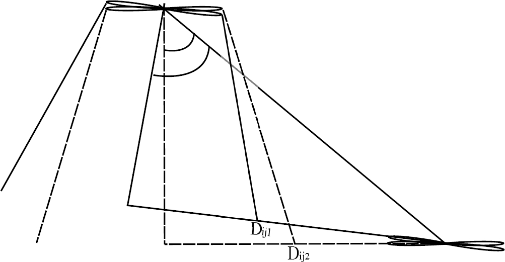
where z is the hub height of the turbine, and z0 is the surface roughness corresponding to the wind farm terrain. The simplest case is when the second turbine is completely immersed into the wake of only one turbine, where the mean velocity is thus given by Equations 1-4. However, this is not always the case (Figure 2):

As it can be seen in this image, three cases could be considered regarding the wake effect:
where Dij, is the distance between the wake center and the center of the affected turbine and r0 the turbine radius. For the first case, it happens that Ashadow,i = A0, and therefore the velocity received by the turbine j its proportional to the the velocity leaving the turbine i. The third case is the easiest, because the wake from turbine i is not affecting the turbine j, and accordingly, Ashadow,i = 0. In the second case, in order to calculate the area Ashadow,i, it is necessary to make some trigonometric computations, considering the wake area as well as the second turbine area:
or alternatively with:
considering that:
A highlight is the fact that Dij is the distance between the wake center and the center of the affected turbine; considering that, as the wind direction changes, such distance changes as well (Figure 3).
Once that Ashadow,i and uij have been calculated with the Equations 1 and 7, the next step is to determine the velocity received by the turbine j:
where Nj represents the number of turbines affecting turbine j and A0 the circular area of each turbine.
Finally, to calculate the power generated by a turbine with a specific wind direction:
In the consulted literature (e.g. [48], [9], [19]), in order to estimate the energy produced by the wind farm, three cases were considered:
Case 1: Uniform wind speed and direction: k = 1, u0 = 8m/s.
Case 2: Uniform wind speed and variable direction: 0 < k ≤ 360, u0 = 8m/s, fk = 0.02778.
Case 3: Variable wind speed and direction: See Table 1.
Table 1 Functions of probability density wind distribution
| u0 = 8m/s | u0 = 12m/s | u0 = 17m/s | |
|---|---|---|---|
| k | fk | fk | fk |
| 0 - 270 | 0.0042 | 0.0084 | 0.0112 |
| 280 | 0.0042 | 0.0107 | 0.0135 |
| 290 | 0.0042 | 0.0126 | 0.0163 |
| 300 | 0.0042 | 0.0149 | 0.0191 |
| 310 | 0.0042 | 0.0149 | 0.0302 |
| 320 | 0.0042 | 0.0195 | 0.0358 |
| 330 | 0.0042 | 0.0149 | 0.0307 |
| 340 | 0.0042 | 0.0149 | 0.0191 |
| 350 | 0.0042 | 0.0126 | 0.0163 |
| 360 | 0.0042 | 0.0102 | 0.0135 |
In the interest of giving a more realistic scenario, the experiments developed in this work only consider the third case. Also, as the final power obtained by the wind farm depends mainly on the entrance velocity for each turbine, and such velocities are at the same time dependent on the shadow area of the wake, we propose to minimize the next objective function:
where:
With respect to λ1, this is a factor empirically selected to penalize the value of the objective function g every time that any other turbine is closer than a security distance to the other turbines in the wind farm (usually, a standard value for such distance is ten times the turbine radius [48]).
3 Differential Evolution
Since the appearing of Genetic Algorithms (GA) [25], several Evolutionary Algorithms (EA) have been proposed including several versions of global optimization (mono-objective), and also for the optimization of problems that include several objective functions; some of those algorithms are the Non-dominated Sortign Genetic Algorithm II (NSGA-II) [38], the NSGA-III [39], the Multiple Objective Particle Swarm Optimization (MOPSO) [42], the Cellular Genetic Algorithm for Multiobjective Optimization (MOCell) [45], and others. Every one of those algorithms are called evolutionary in the sense that their operators are inspired in the evolution theory, which was first proposed by Darwin and later enhanced by Mendel studies [52].
In this article, five variants of an EA, called Differential Evolution (DE), are used to solve the Wind Farm Layout Problem (WFLP). Some comparisons are also presented in order to find which one gives the best result for a given family of problems [58], that are related to the performance and quality of previously found solutions. The DE algorithm was proposed by [56] as a global optimization problem solver, and it has some interesting characteristics: it holds few parameters to tune, it is population-based, it does not use gradient information, and its operators are inspired by evolution, just to mention some of them [16].
3.1 Initialization
The first step in this algorithm consists in the initialization of a population of Np individuals:
where yi ∈ RD and {yu, yl} ∈ RD. yi is a vector that represents a candidate solution and {yu, yl} the upper and lower limits of search space. rand() is a vector of uniformly generated random numbers.
After the initialization, the operators that are proposed for each version make different path searches over the solution space [16]. In the next paragraphs some specific operators that belong to each version are explained.
3.2 Mutation Variations
After the initialization, for each individual in the population a mutant vector is generated. This is achieved in several ways:
considering that r1 ≠ r2 ≠ r3 ≠ r4 ≠ r5 ≠ i are integer numbers, that are randomly obtained from a uniform distribution. ybest is the best candidate solution found so far. The value of F is used as a scaling factor to weight the difference between the selected parents.
These equations represent the five canonical variations proposed by [56]. Even tough there are several other variants of Differential Evolution (DE) [15], a more extensive comparison that considers all of them is out of the scope of this work.
3.3 Crossover
Once the mutant vector is acquired, the next step consists in completing a trial vector:
where 0 < Cr ≤ 1.0, and jrand is an integer random number that ensures that at least one gene from the candidate solution has changed. This scheme is known as binomial crossover; other two crossover versions are the exponential, and the arithmetic recombination. Only the binomial crossover scheme, given by Equation 18, is actually employed in this article.
3.4 Population Update
The final operator of this technique is called selection:
in which the trial vector is evaluated and compared against the original individual. This step is applied over the whole population (synchronous update); in other words, at each iteration both a mutant population, and a trial population are generated. Finally, the operator called population update is applied over the trial population.
The mentioned operators given by Equations Equation 17 - 19 are applied to each individual of the population until a certain criterion is reached, which it is usually a maximum iteration number.
4 Numerical Experiments
4.1 Problem Instances of the WFLP
The methodology adopted in this article, that was used to compare the Differential Evolution (DE) variants, is similar to the one utilized in [33]. In that sense, 25 instances of the WFLP were considered: Nt ∈ [10, 20, 30, 40, 50], with physical terrain limits given by yu ∈ [1000, 1500, 2000, 2500, 3000]. As it can be seen from Nt, the size of the candidate solution changes as the number of turbines changes; this is because each candidate solution is composed by the (pij,qij) coordinates. For example, consider a problem instance with Nt = 10 and yu = 1000, and therefore D = 20; in this case, a possible candidate solution is composed as:
or alternatively as:
whereas the box restrictions are:
and in a more general representation:
Again, it is necessary to remark that the problem’s dimension increases in a twofold proportion with respect to the number of turbines placed into each instance of the wind farm; consequently, the WFLP instances considered in this paper are of 20, 40, 60, 80, and 100 dimensions.
4.2 Parameters Optimization
The term ’meta-optimization’ (also called self-adaptive methodology [47]) is considered a relatively new concept, that consists in using a high level optimization technique to obtain the best tuning parameters of lower level optimization(s) algorithm(s) [14], [60]. By following such idea, in this article the Differential Evolution (DE) version best/1/bin is utilized as the meta-algorithm, and which was manually tuned by following the suggestions given in [41], whereas the lower level algorithms are the five DE variants examined in this work. The fitness function utilized for the meta-optimization is simply the sum of best individuals [60] found after each iteration of the meta-algorithm:
since the limits of the search space are:
and
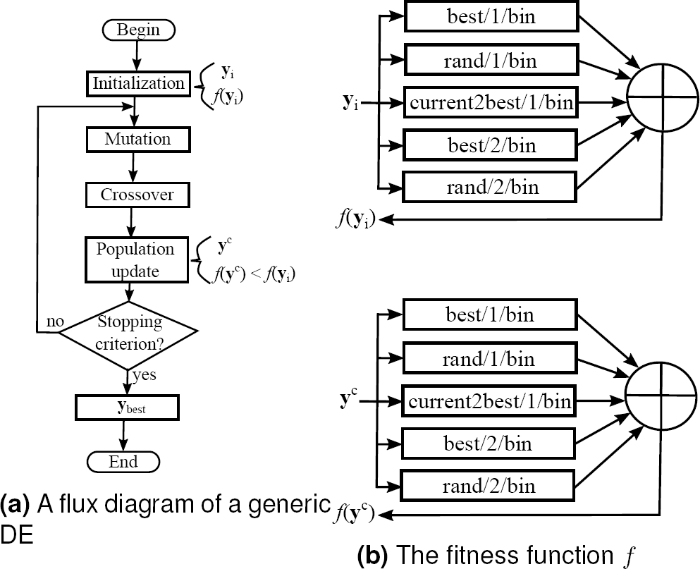
In the meta-optimization process, each candidate solution is a possible combination of the tuning parameters for each DE variant; therefore, the search space has 10 dimensions (D = 10). A simple graphic explanation of the meta-optimization process, utilized in this work, is given in Figure 4. As can be seen, in order to evaluate the fitness function f, every of the five DE algorithms is executed once (200 iterations, Nt = 46 and yu = 2000 [60], with the fitness function g) with the actual candidate solution (e.g. the tuning parameters), and the best individual evaluations are added every run per algorithm (Equation 20). Such process is repeated until the best configuration of parameters is found (Table 2).
4.3 Wind Farm Considerations
In this article it is taken into account the fact that the collocation of each turbine could be anywhere in the offshore wind farm (e.g. [53, 47, 9]) as opposed to other cases where it is divided in an equally spaced grid of cells (e.g. [7, 8, 10]).
As mentioned before, with the idea of making simulations as real as possible, in this paper it is only considered the case when the wind speed and direction are variable [12], according to a certain probability density function. The wind farm remaining parameters are standard values, usually given by other authors in similar studies (e.g. [48]); those values are: z0 = 0.3, z = 60, and CT = 0.88.
Moreover, the objective function is mainly related with the minimization of the shadow areas and its accumulated penalties; in other words, the main idea behind this objective function is to minimize the number of turbines affecting to each turbine in the wind farm. Lets consider a possible configuration, as shown in Figure 5. In this case, two turbines are both partially, and completely immersed into the wake of a third turbine; therefore, the shadow area of the first turbines are respectively accumulated, together with a penalization factor.

4.4 Evaluation and Comparison of Algorithms
In this section are given the considerations with respect to the evaluations of the performance for the five Differential Evolution (DE) variants prior to the experiments made in this work; for example, the utilized algorithms were programmed in Matlab 9.0.0, run on a PC with an Intel i7 multicore processor to 3.4 GHz, and with 16GB of RAM memory.
In terms of the methodology, every algorithm was executed 30 times for each problem instance (200 iterations per run, Figure 6), after which the best results were averaged [33], obtaining 25 results per DE version (Table 3); in order to determine the best algorithm for the WFLP, those results were later statistically compared by means of the Wilcoxon non-parametric test [3, 43].

Table 3 Average best individuals for the 25 problem instances of the WFLP (in kWh)
| Nt | WF size | best/1 | rand/1 | curtobest/1 | best/2 | rand/2 |
|---|---|---|---|---|---|---|
| 10 | 1000X1000 | 8846.81 | 8842.90 | 8848.45 | 8812.75 | 8839.03 |
| 10 | 1500X1500 | 8907.04 | 8908.09 | 8907.26 | 8891.01 | 8910.96 |
| 10 | 2000X2000 | 8944.64 | 8948.59 | 8943.72 | 8927.31 | 8948.54 |
| 10 | 2500X2500 | 8970.86 | 8970.45 | 8969.51 | 8957.80 | 8971.97 |
| 10 | 3000X3000 | 8989.90 | 8986.20 | 8988.10 | 8978.11 | 8987.19 |
| 20 | 1000X1000 | 16847.52 | 16845.48 | 16848.12 | 16724.52 | 16867.48 |
| 20 | 1500X1500 | 17318.15 | 17269.29 | 17289.16 | 17240.88 | 17308.15 |
| 20 | 2000X2000 | 17552.24 | 17511.51 | 17508.70 | 17463.40 | 17504.18 |
| 20 | 2500X2500 | 17665.67 | 17634.01 | 17633.32 | 17617.76 | 17617.71 |
| 20 | 3000X3000 | 17739.49 | 17721.21 | 17713.19 | 17708.64 | 17731.32 |
| 30 | 1000X1000 | 23887.42 | 23824.83 | 23815.34 | 23415.82 | 23834.04 |
| 30 | 1500X1500 | 25089.43 | 24938.36 | 24985.92 | 24878.41 | 24985.90 |
| 30 | 2000X2000 | 25669.91 | 25578.55 | 25555.24 | 25486.11 | 25571.06 |
| 30 | 2500X2500 | 25988.81 | 25906.26 | 25897.38 | 25885.10 | 25947.96 |
| 30 | 3000X3000 | 26180.01 | 26128.43 | 26117.32 | 26109.38 | 26164.00 |
| 40 | 1000X1000 | 29485.65 | 29457.23 | 29380.95 | 28777.05 | 29361.93 |
| 40 | 1500X1500 | 31956.53 | 31871.57 | 31879.86 | 31583.46 | 31925.59 |
| 40 | 2000X2000 | 33203.87 | 33074.22 | 33116.09 | 32976.35 | 33130.64 |
| 40 | 2500X2500 | 33873.82 | 33735.19 | 33734.12 | 33738.25 | 33796.71 |
| 40 | 3000X3000 | 34249.54 | 34206.96 | 34235.98 | 34180.89 | 34210.11 |
| 50 | 1000X1000 | 33726.53 | 33967.76 | 33948.51 | 32780.35 | 33931.54 |
| 50 | 1500X1500 | 37944.01 | 37942.27 | 37863.35 | 37387.27 | 37823.94 |
| 50 | 2000X2000 | 40088.87 | 40046.81 | 39997.65 | 39814.76 | 40071.16 |
| 50 | 2500X2500 | 41333.62 | 41117.88 | 41191.57 | 41016.10 | 41338.35 |
| 50 | 3000X3000 | 42051.30 | 41929.66 | 41950.96 | 41864.38 | 41945.04 |
This test is used when the distribution of data is unknown [17], and also to statistically probe two hypotheses: on one hand, the null hypothesis, which establishes that two samples came from the same experiment, and on the other hand, the alternative hypothesis, that considers that those specimens are significantly different and, therefore, they came from different experiments.
4.5 Results and Discussion
In this section are presented the results obtained by each algorithm. A simple graphic representation of those outcomes is depicted in Figure 7.
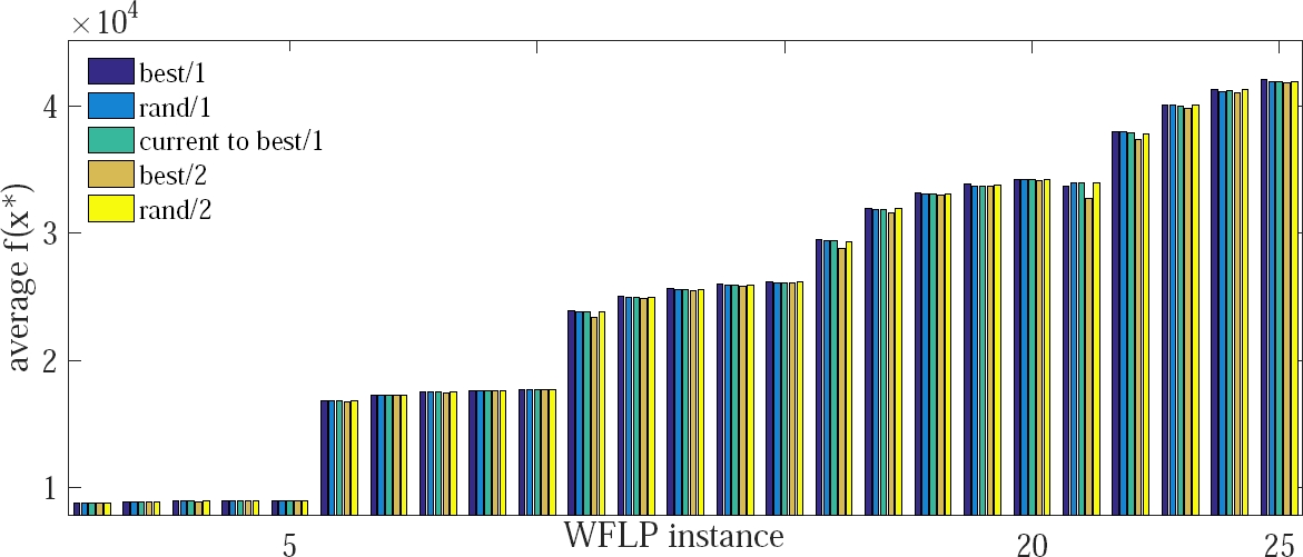
For the first 10 instances, it is clear that each algorithm behaves in a similar fashion; in this case, it is relatively easy for every algorithm to place 10 and 20 turbines into each wind farm, particularly when the terrain’s size increases, which is the case for every Wind Farm Layout Problem (WFLP) instance. However, as the turbines’ number extends to 30, 40, and 50, the problems then become more complicated, and therefore the differences of the algorithms are more evident. From the same graphic, it can be seen that in many instances, the DE/best/2/bin has the poorest performance. Yet, in order to give a detailed statistical explanation to the depicted results (shown in Table 3), the outcomes of the Wilcoxon non-parametric test are displayed in Table 6. As it can be seen after reviewing Table 3, the best technique seems to be the DE version best/1/bin, and therefore, it is statistically compared against the remaining algorithms; according to those results, that algorithm is the best to solve the WFLP, at least for the considered problem instances. In other words, for every pair of algorithms and based on the Wilcoxon non-parametric test, it can be concluded with a confidence of 5% that the algorithm DE/best/1/bin outperforms every other algorithm in the given experimental set, and therefore is the most adequate to tackle the offshore WFLP, at least under the conditions mentioned in this article. Finally, the second best algorithm was selected, which according to Table 3 is the so-called rand/2. That algorithm was compared against the remaining three (Table 6); the results suggest that the performance of the algorithms rand/2, rand/1, and current-to-best/1, is quite similar. In that sense, it can be considered, with a confidence of the 5%, that every algorithm behaves in a similar way for the problem at hand. For the WFLP, it can be considered that DE/best/2 has the poorest efficiency (Table 3-6).
Table 4 List of symbols for the WFLP
| Name | Description |
|---|---|
| a | Axial induction factor |
| A0 | Circular area of each turbine |
| Ashadow,i | Area of the intersection between Aw and Ao |
| Aw | Wake area at distance xij |
| CT | Thrust coefficient |
| Dij | Distance between the wake center and the affected turbine’s center |
| d | Distance between turbine i center and turbine j center |
| Dij | Distance between the wake center and the affected turbine’s center |
| d1 | Distance between the wake center and the radical line center |
| d2 | Distance between the affected turbine’s center and the radical line center |
| fk | Probability density of wind distribution for wind direction k |
| k | Wind direction |
| Nj | Number of turbines affecting turbine j |
| Nt | Number of turbines in the wind farm |
|
|
Power generated by turbine j at wind direction k |
| r0 | Turbine radius |
| rij | Wake radius at distance xij |
| u0 | Free wind speed |
| uij | Reduced wind speed between turbine i and turbine j |
| uj | Wind speed received by turbine j |
| xij | Distance along the wake between turbine i and turbine j |
| z | Turbine hub height |
| z0 | Surface roughness |
| zij | Height of Ashadow,i over the radical line |
| γ | Entrainment constant, also called wake decay constant |
| θω | Angle between rij and Dij |
| θτ | Angle between r0 and Dij |
| λ1 | Penalization factor related with a security distance among turbines |
Table 5 List of symbols for DE
| Name | Description |
|---|---|
| Cr | Crossover factor |
| D | Problem dimension |
| f | Meta-optimization objective function |
| F | Scaling factor of difference |
| g | Shadow objective function |
| Np | Population of candidate solutions |
| (p, q) | Coordinates where a single turbine is placed |
| rand() | Vector of uniformly generated random numbers |
| yi | Vector that represents a candidate solution |
| yu, yl | Upper and lower limits of the search space |
| ybest | Best candidate solution found so far |
|
|
Candidate solutions randomly taken from population |
|
|
Mutated vector |
|
|
Trial vector |
Table 6 Wilcoxon p-values for DE/rand/2/bin against the other DE variants
| best/1 vs. | p-value | Observation |
|---|---|---|
| rand/1 | 0.00054 | Different |
| currenttobest/1 | 0.00049 | Different |
| best/2 | 1.22903 × 10⁻⁵ | Different |
| rand/2 | 0.0022 | Different |
5 Conclusions and Future Work
In this paper is proposed a comparison among five different DE algorithms that are utilized to solve the Wind Farm Layout Problem (WFLP). After running the algorithms several times, it can be statistically stated that the version DE/best/1/bin finds the best results regarding to the quality of the obtained solution. As it has been stated, a possible future venue in the area of Offshore Wind Farm Layout Optimization could be the contrast between other variants of DE, such as hybridizations in order to find the most appropriate algorithm that delivers a better solution for the aforementioned problem.
Even though it has been only mentioned in this article, another established research area in renewable energy is the use of parallel as well as multiobjective optimization approaches [4], [53]; in that sense, a possible extension for this work is the application of several multi-objective algorithms such as the NSGA-II [38], the NSGA-III [39], the MOPSO [42], the MOCell [45], etc., for the WFLP optimization, assuming the objective function that has been proposed in this work. Likewise, the Net Present Value [53], the Energy Yield [49], the Cost of Energy [9], and others can also be considered. Moreover, in order to produce further improvements, the use of more than two objective functions could be potentially achieved by means of using the first two as the functions being optimized, while the remaining are kept as restrictions for the WFLP.

