


 text new page (beta)
 English (pdf)
 Article in xml format
 Article references
 Send this article by e-mail
 Cited by SciELO
  Similars in
SciELO
Similars in
SciELO 
 Permalink
1 Introduction
Breast cancer screening is the medical procedure of asymptomatic, apparently healthy women in an attempt to achieve an earlier diagnosis [36]. Mammography is the most common screening method since it is relative fast, cheap and widely available. This imaging process use a very low ionizing radiation dose to examine the human breast, due to the resulting image has low contrast and the different parts of the breast are hard to distinguish, in particular, detecting masses and microcalcifications requires years of medical training. The anomalies vary in size and shape, and might be located in dense tissues making their detection more difficult. Also, breast tissues are different in younger and senior women [18]. Conventional methods like CLAHE, Unsharp Masking, median filtering and Gaussian filtering don’t have enough visual quality to help a radiologist [1].
The wavelets approach has been widely used in digital mammography with satisfactory results [1]. Nevertheless, there are few works that establish a procedure to choose the wavelet base and the combination of decomposition levels that must be processed to effectively increase the contrast in mammographies [5]. This paper proposes a methodology to select the decomposition levels to be process in wavelet-based algorithms. A contrast improvement is performed by modifying the wavelet coefficients using the Local Correlation method in a logarithmic framework [4, 22]. Quantitative contrast measures [34] and Principal Components Analysis [15] are used to select the best combination of decomposition levels.
The rest of the paper is structured as follows. Section 2, introduce the Discrete Wavelet Transform and the Logarithmic Image Processing framework. In Section 3, we propose an algorithm based on the Logarithmic Discrete Wavelet Transform for mammography contrast enhancement. In Section 4 we present a methodology to select wavelet base and combination of decomposition levels to be processed for a good contrast enhancement of breast anomalies. The experimental setup is described in Section 5. In Section 6, the results are discussed. Some remarks and conclusion are given in Section 7.
2 Discrete Wavelet Transform and the Logarithmic Image Processing Framework
A gray-level image is a function
The Discrete Wavelet Transform (DWT), derives from the discretization of the scaling factor
A discrete scaling function
with these two functions constituting a Riesz basis [25].
The computation of the DWT can be expressed by the approximation coefficients
with
According to Mallat [21], the 2-D wavelet is defined as:
The whole image
The DWT provides a ‘measure of similarity’ between the image and the mother wavelet around the pixel
Generally, the wavelet-based algorithms have three main stages. First, the image is decomposed in horizontal, vertical and diagonal detail coeffi-cients and the approximation coefficients. At this stage is important to select the wavelet base and levels of decomposition to be process. Different approaches for wavelet base selection has been addresses in [29, 11]. Cheng et al. proposed an automatic wavelet base selection to enhance contrast of natural images [5]. In this contribution we study a way to select the proper wavelet base to improve contrast in mammography images, also related with the type of anomaly; to our knowledge this task hasn’t been done yet.
Usually, in the literature all decomposition levels are processed until a selected one (each wavelet base have a maximum level of decomposition). A low decomposition level implies more efficiency of the wavelet decomposition algorithm. In previous work we founded that its not necessary to process all the levels to enhance the contrast [37]. Due to, in our proposal we include a methodology to select levels of decomposition to be process. In our bibliography study we don’t find evidence of similar approach.
In the second stage of wavelet-based algorithms, the detail coefficients of selected decomposition levels are modified to improve the contrast. Finally, applying the inverse wavelet transform (IDWT), the enhanced image is obtained.
There are several methods for modifying the detail coefficients. A group of algorithms uses a non-linear function that follows certain criteria established by Laine and Song [20]. Some methods apply heuristics over the wavelets coefficients, e.g. Simple, Threshold, Correlation and Local Correlation methods [22]. In [37] we demonstrated that the most effective method is the Local Correlation. It is based on the following theoretical concept: coefficients that retain high values at different decomposition levels must be correlated and therefore are part of an anomaly. For detecting high values are only considered the coefficients of a neighborhood, hence the name local. This concept was presented by Stefanou et al. [35] and Chen et al. [4]. This method achieves a good increment of the contrast of the masses and other elements such as the pectoral and the edge of the breast.
2.1 Non-Linear Models for Image Processing
The non-linear models of image processing (NIP, also known as Logarithmic Models), are an alternative to the classical image processing, based on floating-point arithmetic, because this approach has the limitation of truncating the sum of pixel values over the limit. These NIP models modify the basic operations over the pixel intensities. The superiority against classical methods has been proved in [10, 17].
NIP models represent an image using an algebraic structure, so it performs operations different to the classical ones (point-to-point).
The mathematical construction of a NIP model starts by the definition of the operational laws (ad-dition and multiplication by scalar), or equivalently finding a generating function (isomorphism), that represents the definition of the model in a real algebraic structure [10]. What distinguishes the models is the isomorphism, since it determines the operations of the algebraic structure. There are several NIP models, but in the experimentation performed in this contribution the S-LIP model [26] was used.
2.1.1 Symmetric Logarithmic Image Processing Model
The Symmetric Logarithmic Image Processing Model (S-LIP), was proposed by Navarro et al. [26] to overcome the disadvantages of previous models with respect to symmetry and its visual meaning.
This model defines the following isomorphism
with the inverse:
Navarro et al. use the Logarithmic Discrete Wavelet Transform (LDWT), and S-LIP model in compression, edge detection and noise suppres-sion in images [25].
3 Logarithmic Discrete Wavelet Transform for Contrast Enhancement in Mammography
The logarithmic wavelet was introduced by Courbebaisse et al. in 2002 [6]. In their paper they prove the advantages of using this type of wavelet to solve problems like detection of singularities. The idea behind logarithmic wavelets is to dilate and translate a wavelet function in a non-linear way. This kind of wavelets are superior to the classic ones because their amplitude changes logarithmically and remain bounded [25].
The S-LIP mother wavelet
where
Then,
where
The three directional S-LIP wavelet are defined as:
The logarithmic wavelet decomposition of image
The scalar product in S-LIP model is defined as:
As we present, the LDWT can be defined using the non-linear operations of the model, however we used another approach. This approach consists in apply
The algorithm proposed in our contribution uses LDWT in a S-LIP model and achieve contrast enhancement through modifying wavelet coefficients with Local Correlation method, as shown in Figure 1.

4 Statistical Analysis for Wavelet Selection
In this section we propose a methodology for wavelet selection, i.e. select the wavelet base and the combination of decomposition levels to be processed. This approach needs the wavelet decomposition of an image for a set of wavelet bases and all possible combinations of decomposition levels, i.e. the power set of {1, 2, 3, maximum level of decomposition-1}. Then, a modification of wavelets coefficients is performed in order to increase the contrast. Finally, we obtain the reconstructed image through IDWT, and a quantitative quality measure is computed on it.
The experimentation presented in this research apply LDWT with S-LIP, model to an image up to the highest decomposition level using a set of wavelet bases. After that, modify the wavelet coefficients by means of the Local Correlation method. Contrast enhancement quality measures based on regions of interest are computed for all the anomalies present in the image.
According to the type of anomaly the best wavelet base was selected following different points of view namely: quality measure, descriptive statistics, visual results, and experiences on wave-let selection presented in reviewed bibliography.
Having the best wavelet base, we choose the decomposition level to be processed through a Principal Components Analysis (PCA) [15], performed to the data fetched from each basis where each column is a different combination of decomposition levels and each row represents the value of the quality measure matching each represented reconstructed image.
PCA reduces the data dimension based on the data variance allowing the visualization of high dimensional data, correlated variables, and more significant variables for describing data. This technique center data with respect to the data mean and then calculates the co-variance matrix [15].
PCA allows us to do the loadings plot where the variance of each combination of decomposition levels is shown. The interpretation of this plot enable to know the behavior of level combinations for contrast enhancement.
The module of loadings vectors represents the deviation of each combination with respect to the data mean. The cosine of the angle between these vectors denote the correlation between the variables that its characterize. An angle near to 0o or 180o means co-linearity (redundancy), whilst an amplitude of 90o and 270o degrees imply low correlation.
The Manhattan plot [7], is another way to interpret the variance of each level combination and complements the results of the loadings plot. This plot consists on a grid which rows are the principal components considered and the columns are the variables of the model (combinations of decomposition levels in this paper). Each cell of the grid have a gray intensity corresponding to explained variance of each variable in the selected component. The black color means 0% explained variance and white represents 100% [31].
We considered the two principal components if these components captures more than 50% of the data variability. Then, we get the combinations that capture more than 90% of the variability per each reconstructed image in the first principal component.
A combination of levels is called “suitable” if it displays the highest variance, the lowest feasible level and the fewest amount of levels to be processed. This criterion is justified because wavelet transform is more efficient if the decomposition is performed to a low level [21]. The obtained combination of decomposition levels allow us to achieve the best contrast improvement according to the quantitative quality measure used.
5 Experimental Setup
The algorithm was tested on 94 sub-images of the image 22670465 of INbreast data set [23]. This image was selected because it contains most diverse set of anomalies of the data set (one mass, one spiculated region, one cluster and 92 calcifications). In this image, anomalies called asymmetry and distortion are not present.
In the used data set each anomaly is annotated using a contour for masses and calcifications and a circle for spiculated regions and clusters.
5.1 Contrast Enhancement Quality Measures
A region of interest (ROI), is formed by a foreground that contains the anomaly, and the background that comprises the surrounding tissue. This construction reflects human visual perception as it perceives an object considering the environment where it is placed. The ROI’s based measures quantifies the contrast of a mammogram’s region chosen by the radiologist or defined automatically.
The INbreast’s contours by anomaly was considered as ROI’s foreground. Since a ROI can vary in forms and size, a flexible background contour is needed. The adaptive margin for this contour was calculated according to the algorithm proposed by Mudigonda et al. [24].
In this paper, the contrast enhancement quality was quantified using Contrast Improvement Index (CII) [30] and Combined Enhancement Measure (CEM) [34]:
CII capture the gain of contrast between original and processed images, it is always positive, and values greater than the unit are considered like a sign of good contrast improvement [32, 30].
CEM combine other three measures: Dis-tribution Separation Measure
DSM quantifies the overlapping between the anomaly and the surrounding tissue,
6 Results and Discussion
The experimentation was split up in the following steps. First, we apply LDWT with S-LIP model to the image up to the highest decomposition level using the following wavelet bases considered in PyWavelets [42]: Haar, Daubechies 1-20, Symlets 1-20, Coiflets 1-5, Biorthogonal 1.1-6.8, Reverse Biorthogonal 1.1-6.8 and Meyer. After that, we modified the wavelet coefficients by means of the Local Correlation method for all possible combinations of decomposition levels.
The behavior of the CII measure in the quality of the image contrast enhancement obtained by different wavelet bases shown low dispersion with respect to the central value 1.0. Although, we observed different behaviors for different type of anomalies (in parentheses we put the values of the measure): for the masses a meaningful contrast enhancement was achieved by the wavelet bases Biorthogonal 2.2 (3.51), Daubechies 3 (3.48) and Symlets 3 (3.48) and for spiculated regions and calcifications the worst results are attained by the Biorthogonal 3.1 (0.14), Reverse Biorthogonal 3.1 (0.55) and Haar (0.55) bases. Also, with this measure we obtained similar behavior for a group of wavelet bases, e.g. in a first group the bases Coiflet 3, Coiflet 4, Coiflet 5 and Meyer; in a second group the bases Daubechies 10-20; and in a third group the bases Symlets 7-20.
In Figure 2, the behavior of some selected wavelet bases is shown, and in Figure 3 we illustrate the ROIs of the three best and worst results of the measure CII with the corresponding wavelet bases and decomposition levels.


The CEM measure gives better results when their values are positive and close to zero. Very poor results are obtained for the wavelet bases Reverse Biorthogonal 1.1 (33.53), Haar (33.46) and Biorthogonal 1.1 (33.42). The best contrast increments for this measure were achieved for the bases Reverse Biorthogonal 3.3 (1.33), Biorthogonal 3.1 (1.33) and Biorthogonal 2.2 (1.34).
In this case we also observed a similar behavior for group of wavelet bases, e.g. Coiflet 3, Coiflet 4, Coiflet 5 and Meyer in a first group; Daubechies 10-20 in a second group; and Symlets 7-20 in a third group.
In Figure 4 we illustrate the behavior of the measure CEM for a selected group of wavelet bases. In Figure 5, ROIs of the three best and three worst results of the measure CEM with the corresponding wavelet bases and decomposition levels are shown.


We calculated the average of the measures CII and CEM for each anomaly and for each wavelet base. Putting all this curves together we can observe the behavior of a specific wavelet base regarding all type of anomalies, as you can see in Figures 6, 7 and 8.


With respect to measure CII, the contrast enhancement for the calcifications was poor on average, See Figure 6. For the masses, the contrast was always increased except for the Reverse Biorthogonal 3.1, in fact this was the type of anomaly with higher values for the measure. For the cluster anomaly, the higher contrast enhancement were scored by wavelet bases Biorthogonal 1.3, Biorthogonal 3.1 and Reverse Biorthogonal 1.3, and the worst results were obtained by Biorthogonal 1.1, Haar and Reverse Biorthogonal 1.1. In the case of the spiculated regions, the best values for this measure were achieved with the Biorthogonal 1.1, Daubechies 1 and Reverse Biorthogonal 1.1 bases, reaching its lower value for the Biorthogonal 3.1 basis (See Figure 7).
In Figures 9 and 10 we show in the diagonal the ROIs, for each type of considered anomaly, processed by the wavelet base which produce the best contrast enhancement according to quality measures CII and CEM, respectively. In each row of both figures the same ROI is processed by the wavelet bases used successfully for the rest of the anomalies. This way we can know if we get, with the same wavelet base, good results to different anomalies.


Although, the visual results do not match the successful values of the quality measures, Figure 11 shows a selection of good visual results for a ROI corresponding to each one of the four types of analyzed anomalies.

In Figure 12, as you can observe we have markers with different shapes, indicating the wavelet base and different colors for each type of anomaly. The horizontal axis refer to the values of the CII measure and the vertical one denote the values of the CEM measure. The optimal location in this graphic would be as close as possible to the horizontal axis and as far as possible to the vertical axis, which means small values of CEM and large values of CII. As it can be seen, the points are far from this region. The best values are below

The quality measures for the enhancement do not provide enough information on their own for the best base selection for improving the contrast. According to research in the literature, Drukker et al. [9] used Biorthogonal 6.8 and Bhateja & Devi [1] uses the Daubechies 6 wavelet basis for the detection of microcalcifications on mammography images. Our experimentation shows that the average value of the CII measure for this wavelet basis isn’t good, nevertheless the value of the CEM measure is low. Visual results confirm the effectiveness of the basis for increasing the contrast on this kind of anomaly. Zhuangzhi et al. presented an Approximation Weighted Detail Contrast Enhancement (AWDCE) filter [43] for detecting masses by the Daubechies 20 wavelet base. However, no well defined analytic approach has been applied for determination of the level of decomposition using Daubechies 20. Schebesch et al. [33] and Vikhe and Thool [40] used Haar basis for detection of masses. Zanchetta et al. used the Daubechies 8, Symlet 8 and Biorthogonal 3.7 bases for classifying masses in normal or abnormal through supervised learning, achieving the best results with Biorthogonal 3.7 [8]. In our experimentation, this basis give the best results for the mass: on average, the values of the CII are higher than the unit and the values of the CEM measure are close to 7. The visual results of the enhancement are successful. Cheng et al. used wavelet bases Symlets 4, Symlets 9, Symlets 12 and Symlets 20 for increasing the contrast of natural images [5]. All these bases display good results visually, the values of the measures are similar and satisfactory. Except for the work of Cheng et al., the choice of these bases is empirical and doesn’t provide any statistical information that compares a choice with a greater number of bases nor a methodology is provided to pick up the decomposition levels to be processed.
Based on previous information and on each wavelet basis characteristics, we decide to study how to select the set of decomposition levels that attain a good increase in the contrast, matching both quality measures and ROIs visual content. The following bases were chosen: the Daubechies 12 for calcifications, Symlets 12 for cluster, Biorthogonal 2.2 for masses and Reverse Biorthogonal 1.3 for spiculated regions.
Then PCA was applied to the rotated data (See Section 4). Figures 13 and 14 shows the loadings corresponding to Daubechies 12 and Biortogonal 2.2 bases. In Figure 13 meaningful differences are noticeable amongst three groups of combinations of decomposition levels: combinations on the first quadrant, combinations on the fourth quadrant and the rest of the combinations. The more pronounced differences (given by the almost orthogonality of the loadings) are shown in the combinations of the first and fourth quadrant. In Figure 14, a combination of levels remarkably distinguishes from the rest stands out.

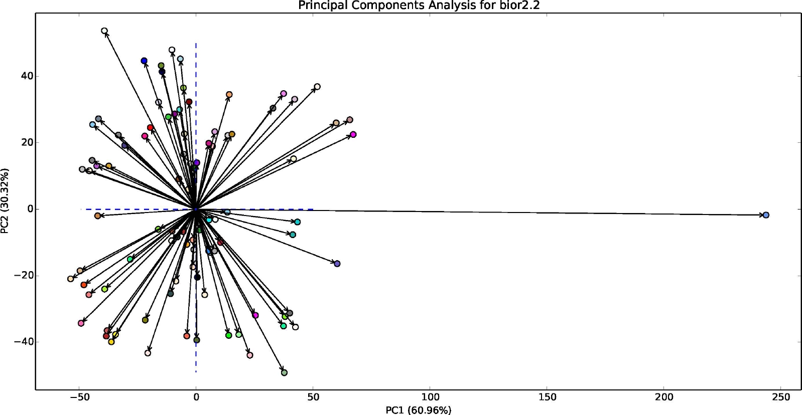
Figure 15 shows the Manhattan plot for the selected bases according to CEM measure. It can be noticed that two principal components were enough in order to represent the whole data variability.

Applying the criterion for the “suitable” levels combination we get (3, 6) for Daubechies 12 and Symlets 12, and (1, 2, 3, 4) combinations for Biorthogonal 2.2 and Reverse Biorthogonal 1.3.

Fig. 16 Results of the proposed algorithm for some ROIs according to the selected wavelet basis and combination of decomposition levels
In Figure 16 we illustrate that the proposed algo-rithm with the selected bases and “suitable” levels combination is successful only for calcifications and masses.
7 Conclusions
Conventional contrast enhancement methods do not work properly in mammography images. The techniques based on wavelet transform have shown their capability for the detection of anomalies that can occur in the mammogram allowing the increase of its contrast.
The presented algorithm, LDWT with S-LIP model and modification of detail coefficients using Local Correlation method, has better results increasing the contrast of calcifications and masses, although it is able to improve the contrast of the rest of the anomalies. Values of the quality measures do not always correspond to the visual results because the process heavily depends on the choice of ROI and the measure of quality used.
As result of the experimentation performed the best wavelet bases were Daubechies 12 for calcifications, Symlets 12 for cluster, Biorthogonal 2.2 for masses and Reverse Biorthogonal 1.3 for spiculated regions. Also, a methodology was proposed to select the combination of decomposition levels to be processed. This procedure consists of performing PCA on the data by taking the values of the CEM measure.
The variability of the data using Manhattan plots was studied and an algorithm was proposed to determine the “suitable” combination of levels. For the masses and calcifications the “suitable” combination was
The ROI’s definition is an important factor to explain the poor contrast improvement of the rest of the anomalies.

