1 Introduction
The propositional μ-calculus is a modal logic with least and fixed-point operators, expressively corresponding to the monadic second order logic MSO [9]. This logic is known to subsume many temporal, program and description logics such as the Linear Temporal Logic LTL, the Propositional Dynamic Logic PDL, the Computation Tree Logic CTL and ALC
reg
, which is an expressive description logic with negation and regular roles [4]. Due to its expressive power and nice computational properties, the μ-calculus has been extensively used as a reasoning framework in a wide range of domains, such as program verification, knowledge representation and concurrent pervasive systems [4]. In concurrent pervasive systems, logic-based reasoning frameworks have been successfully tested in context-aware scenarios [2, 3]. In this paper, we propose a reasoning (satisfiability), algorithm for the μ-calculus with converse, where formulas are interpreted over finite unranked tree models. The algorithm is based on a depth-first search, and its complexity is optimal, that is, exponential time with respect to the input formula. We also describe an implementation of the algorithm.
XPath is the standard query language for semi-structured data (XML). This query language also takes an important role in many XML technologies, such as, XProc, XSLT and XQuery. Although the full XPath query language is known to be undecidable [15], the μ-calculus with converse has been successfully used as a reasoning framework for the navigation core of XPath, known as regular path queries [5, 7]. We also describe a logic characterization of regular path queries in terms of μ-calculus formulas. Since the logic is closed under negation and the proposed algorithm is optimal, our implementation can be used for optimal standard reasoning (emptiness, containment and equivalence), of regular path queries.
1.1 Related Work
The validity/satisfiability problem of the μ-calculus is in EXPTIME-complete [4]. Furthermore, in [4], several μ-calculus extensions are studied: converse programs (modalities), allows expressing backwards (past) properties; nominals are special formulas to denote individuals; and graded modalities express numerical constraints on node occurrences. The μ-calculus extended with either converse and nominals, converse and graded modalities, or nominals and graded modalities are also complete in EXPTIME. However, the extension consisting of all three features (nominals, converse and graded modalities), known as the fully enriched μ-calculus, leads to undecidability.
These results were obtained by the development of corresponding automata machinery, which was not reported to be implemented. Tableau-based decision algorithms for the μ-calculus with converse and nominals, converse and functional modalities (restricted graded modalities), and nominals and functional modalities are presented in [13].
The complexity of these algorithms is also single exponential time. Implementations of the algorithms are also described. In contrast with this work, where the logic formulas are interpreted over Kripke structures (graphs), in the current paper, we propose a satisfiability algorithm for μ-calculus with converse over finite unranked trees.
A decision algorithm for the monadic second order logic, equally expressive as the μ-calculus, was proposed in [8]. This algorithm, based on automata, was shown useful in practice on the verification of hardware and programs, however its complexity is non-elementary.
In [5], it is also introduced an automata machinery for the μ-calculus with converse over trees. This machinery supports model checking in linear time and decidability in exponential time. Also in this case, implementation is not reported. Another EXPTIME decision algorithm for this logic, the μ-calculus with converse over trees, is presented in [7]. This algorithm is based on a breadth-first search in the style of Fischer-Ladner [6]. In the current paper, we also propose a Fischer-Ladner algorithm, but based in a depth-first search. Experiments show competitive results with respect to the breadth-first search algorithm.
XPath has been widely studied before from the formal perspective [15, 5, 7].
Although it is known that the full language is undecidable [15], several complexity results have been obtained for decidable fragments. The navigation core of XPath, containing all features to allow multi-directional navigation (children, siblings, ancestors, descendants, etc.), is known as regular path queries. Emptiness, containment and equivalence of regular path queries are known to be in EXPTIME [5].
The sole known reasoning solver reported so far for regular path queries can be found in [7]. In this paper, we also describe several reasoning experiments for regular path queries. These experiments show that our implementation is competitive in running time with respect to the other known implementation.
1.2 Outline
We first introduce the μ-calculus with converse modalities in Section 2. Then in Section 3, we introduce the notion of Fischer-Ladner trees, which is the syntactic structure constructed by the satisfiability algorithm, which is described in detail in Section 4. Also in this section, it is shown that the algorithm is correct (sound and complete) and optimal (EXPTIME). In Section 5, we describe a linear characterization of regular path queries in terms of μ-calculus formulas. We also report in this section several query reasoning experiments. We conclude in Section 6, with a summary of the paper together with a brief discussion of further research perspectives.
2 The μ-Calculus on Trees
In this section, we introduce the μ-calculus with converse. Formulas are interpreted over finite unranked trees. The alphabet is considered by two sets, PROP and MOD, where PROP is a set of proposition and MOD={1,2,3,4}, is the set of modalities.
Definition 1 (Syntax). The set ofμ-calculus formulas is defined by the following grammar:
φ::=p|X|¬φ|φ∨ψ|〈m〉φ|μX.φ
where p is a proposition, m a modality, and X is a variable.
We assume variables can only occur bounded and in the scope of a modality.
Formulas are interpreted as subset nodes in unranked trees. Propositions are used as labels for nodes, negation (¬), is interpreted as set complement, disjunctions are interpreted as set union. We write ϕ∧φ instead of ¬(¬ϕ∨¬φ).
Modal formulas 〈m〉ϕ holds in nodes where there is an m-adjacent node supporting ϕ. The least fixed-point is intuitively interpreted as a recursion operator.
We now present the tree structures defined in style of kripke.
Definition 2 (Tree structure). A tree structure, or simply a tree, is a tuple (N, Rm, L) where:
we give a formal description of the semantic of a formula, where Var is a set of fixed-point variables, 2N is the power set of nodes:
sust(V,K,X,φ):=V′(Y)=V(Y) where Y≠X.
sust(V,K,X,φ):=V′(Y)=〚φ〛VK where Y=X.
Definition 3 (Semantics). Consider a tree K and a valuation V:Var↦2N, where Var is a set of variables. The semantics of the formula is defined as follows:
〚p〛VK = {n|p∈L(n)},〚¬φ〛VK = N\〚φ〛VK,〚φ∨ψ〛VK = 〚φ〛VK∪〚ψ〛VK,〚〈m〉φ〛VK = {n|R(n,m)∩〚φ〛VK≠0},〚X〛VK = V(X),〚μX.φ〛VK = ∩{N′|〚φ〛VK [μX.φ/X]⊆N′}.
A formula ϕ is satisfiable, if and only if, there is a tree (model), such as the interpretation of ϕ over the tree is not empty, that is 〚ϕ〛VK≠∅.
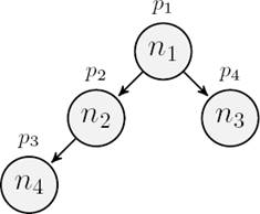
Example 1. In Figure 1, there is a graphical representation of tree model. Consider for instance the following formula:
〈1〉p2∧p1,
This formula selects nodes names p1 with a child named p2. In Figure 1, this formula holds in n1. Recursive navigation can be expressed with the fixed-point:
μX.(p3∨〈1〉X)∧〈1〉p2∧p1.
This formula holds in a p1 node with a descendant p3 at node n4 and a child p2 at node n2. In Figure 1, this formula also holds in n1.
3 Fischer-Ladner Trees
The satisfiability algorithm builds a syntactic version of tree structures, called Fischer-Ladner trees [6], where nodes are sets of subformulas. In this Section, we define this notion of trees.
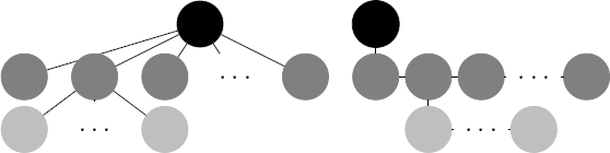
There is a well-know bijection between n-ary and binary trees: one relation is for the first-child (parent), and the other for the following (previous) sibling. In Figure 2, there is a graphical representation of this bijection. Hence, without loss of generality, for technical convenience, we work on binary trees. Also, modal formulas should be re-interpreted:
— 〈1〉φ holds in nodes where its first child supports φ;
— 〈2〉φ is interpreted in nodes where φ holds in its following (right) sibling;
— 〈3〉φ stands where φ is the parent; and
— 〈4〉φ where φ is the previous (left) sibling.
We also consider formulas in negation normal form only: negation only occurs in front of propositions and formulas 〈m〉⊤, where ⊤ stands for p∨¬p. We then define the following function.
nnf(X)=¬X,nnf(p)=¬p,nnf(φ∨ψ)=nnf(φ)∧nnf(ψ),nnf(〈m〉φ)=〈m〉nnf(φ)∨¬〈m〉⊤,nnf(μX.φ)=μx.nnf(φ)[X/¬X].
We then define the negation normal form of a formula, as the resulting formula of replacing negations ¬φ with nnf(φ).
Some notions are required before introducing Fischer-Ladner trees.
Definition 4. We define a binary relation RFL on formulas with i=1,2:
|
RFL(φ,nnf(φ)),RFL(〈m〉φ,φ),RFL(φ1∨φ2,φi).
|
RFL(φ1∧φ2,φi),RFL(μX.φ,φ[μx.φ/X]),
|
Definition 5 (Fischer-Ladner Closure). Given a formula φ , the Fischer-Ladner closure of φ is defined as FL(φ)=FL(φ)k, where k is the smallest positive integer satisfying FL(φ)k=FL(φ)k+1, where:
FL(φ)0={φ},FL(φ)i+1=FL(φ)i∪{ψ′|RFL(ψ,ψ′),ψ∈FL(φ)i}.
We now define the lean set for the syntactic nodes. This set is intuitively composed by the propositions and modal subformulas of the input formula. The propositions are used to name the nodes, and modal subformulas give the topological information of candidate trees.
Definition 6 (Lean). Given a formula φ and a proposition p′ not occurring in φ , the lean of φ is defined as follows for all m∈MOD :
lean(φ)={p,〈m〉φ∈FL(φ)}∪{p′,〈m〉⊤}.
Example 2. Consider the following formula:
φ=〈1〉〈1〉¬p1∧〈1〉¬p1∧¬p1∧μX.(p1∨〈1〉X)∧〈2〉p2∧p3.
The lean of φ is defined as follows:
lean(φ)={p1,p2,p3,〈1〉¬p1,〈1〉〈1〉¬p1,〈1〉μX.(p1∨〈1〉X),p′,〈2〉p2,〈1〉⊤,〈2〉⊤,〈3〉⊤,〈4〉⊤}.
We are now ready to define nodes in Fischer-Ladner trees.
Definition 7 (Nodes). Given a formula φ , a node in Fischer-Ladner trees is defined as subset of lean(φ) , such as:
— it contains at least one proposition;
— if 〈m〉ψ occurs in it, also 〈m〉⊤ does;
— both 〈3〉⊤ and 〈4〉⊤ do not occur in it.
Example 3. Consider the same formula and corresponding lean as in Example 2. We then define the following nodes:
— n1:{p3,〈1〉μX.(p1∨〈1〉X),〈1〉¬p1,〈1〉〈1〉¬p1,〈2〉p2};
— n2:{p′,〈1〉¬p1,〈1〉μX.(p1∨〈1〉X)};
— n3:{p′,〈1〉μX.(p1∨〈1〉X)};
— n4:{p1};
— n5:{p2}.
And we now finally define Fischer-Ladner trees.
Definition 8 (Fischer-Ladner Tree). We inductively define Fischer-Ladner trees as follows:
— The empty tree ∅ is a Fischer-Ladner tree; and
— (n,X1,X2) is a Fischer-Ladner tree, provided that n is a node (called the root), and X1 and X2 are Fischer-Ladner trees.
when clear from context, we often write simply a tree instead of a Fischer-Ladner tree.
Example 4. Consider the nodes in Example 3. We then define the following tree:
T=(n1,(n2,(n3,(n4,∅,∅),∅),∅),(n5,∅,∅)),
Figure 3, ilustrates the tree.
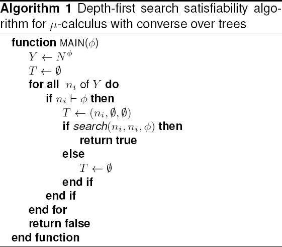
4 Depth-First Search Based Satisfability Algorithm
In this section we describe satisfiability algorithm of μ-calculus based on depth-first search. The Algorithm 1 decides whether a formula is satisfiable or unsatisfiable. In the main function the algorithm creates the required nodes. Then the nodes are iterated. The satisfiability algorithm builds the tree starting from the node that satisfies the formula. This node is used as a candidate and from it begins the construction of the tree. Once the node is selected, the algorithm enters the search function.
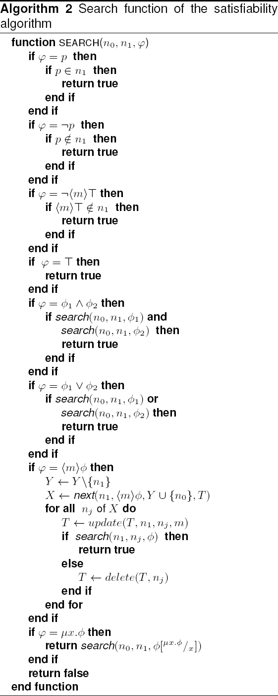
The Algorithm 2, shows the search function. When the formula is p,⊤,¬p or ¬〈m〉⊤, then, the algorithm evaluates the satisfiability of the node and returns true. If it contains fixpoint, then, algorithm makes its expansion and called the function search. The cases for disjunction and conjunction, the algorithm invokes the search function on both sides. When the formulas have the form of modality, it searches the next node. The formula can contain modalities 〈1〉,〈2〉,〈3〉 or 〈4〉.
The current node is deleted from the list of nodes, the algorithm obtains a list of the following nodes with the next function, the node list is iterated and the tree is updated. It is called the search function, if it returns false, thus, the next node is removed from the tree. Each time a node is added, it is passed to the status used and it can not be reused in subsequent levels of the tree, avoiding in such a way to build an infinite tree. If there are not more nodes to search, then the algorithm returns false. The algorithm ends when all nodes have been traveled or the tree is built.
Now we define when a formula is satisfiable.
Definition 9. Given a formula ϕ and a node n , we define the satisfiability n⊢ϕ as follows:
n⊢⊢,φ∈nn⊢φ,n⊢φn⊢φ∨ψ,n⊢ψn⊢φ∨ψ,φ∉nn⊢¬φ,n⊢φ n⊢ψn⊢φ∧ψ,n⊢φ[ μx.φ/x]n⊢μx.φ.
The Δm function is responsible for verifying the union of one node with respect to another node through a modality m. Where n′ is possible to join node, n1 the current node, m are modalities 〈1〉 or 〈2〉, m¯ are reverse modalities 〈3〉 or 〈4〉 and 〈m〉φ modal formula.
Definition 10. Given two nodes n , n′ and formula φ , it is determined that these nodes are consistent with respect to the formula Δm(n,n′) where m∈{1,2,3,4} , if and only if modal formulas 〈m〉φ1,〈m¯〉φ2∈lean(φ) , it states the following:
Example 5. Given the formula φ=〈1〉〈1〉¬p1∧〈1〉¬p1∧¬p1∧μX.(p1∨〈1〉X)∧〈2〉p2∧p3. used in Example 2 the unions are the following:
—Δm(n1,n2),
—Δm(n1,n5),
—Δm(n2,n3)
—Δm(n3,n4)
where n1={p′,〈1〉μX.(p1∨〈1〉X),〈1〉¬p1,〈1〉〈1〉¬p1,〈2〉p2,p3} , n2={p′,〈1〉¬p1,〈1〉μX.(p1∨〈1〉X)} , n3={p′,〈1〉μX.(p1∨〈1〉X)} , n4={p1} and n5={p2} .
These nodes are consistent because the child nodes contain the witnesses of the modal formulas.
The next function obtains the set of nodes subsequent to a candidate node. This function is defined by a triplet of elements (n,〈m〉φ,Y). Where n is the current node, 〈m〉φ modal formula, Y the set of nodes unused and T is tree.
Definition 11 (Nodes). Given a tree T , the nodes function is defined as follows:
A node Tn is denoted as follows:
Definition 12 (SubTree). The subtree T′ of a given tree T(T′⊆T) is defined as follows:
Definition 13 (Root). The root(T) function takes the tree as input and returns a node root of the tree.
—root(∅)=∅,
—root((n,T1,T2))=n.
Definition 14 (neighborhood). Given a tree T and node n , the neighborhood function obtains adjacent nodes. Considering that exist trees T′, T1 and T2 :
— parent(n,T)=n′ such that, (n′,Tn,T′)⊆T,
— child(n,T)=n′ such that, (n,(n′,T1,T2),T′)⊆T,
— ps(n,T)=n′ such that, (n′,T′,Tn)⊆T,
— fs(n,T)=n′ such that, (n,T′,(n′,T1,T2))⊆T,
— neighborhood(n,T)={parent(n,T),child(n,T),ps(n,T),fs(n,T)}.
Definition 15 (Delete). Given a tree T and node n , the node is removed of tree, the Delete function is defined as follows:
—delete(∅,n)=∅,
—delete((n,T1,T2),n)=(∅,T1,T2),
—delete((n′,T1,T2),n)=(n′,delete(T1,n),delete(T2,n)),
where n≠n′.
Definition 16 (Update). Given a tree T, two different nodes n and n′ and a modality m, the Update function is defined as follows:
When n′∉nodes(T),
-update((n,T1,T2),n,n′,3)=(n′,(n,T1,T2),∅),
-update((n,T1,T2),n,n′,4)=(n′,∅,(n,T1,T2)),
-update((n,∅,T2),n,n′,1)=(n,(n′,∅,∅),T2),
-update((n,T1,∅),n,n′,2)=(n,T1,(n′,∅,∅)),
-update((n″,T1,T2),n,n′,m)=(n″,update(T1,n,n′,m),update(T2,n,n′,m)),
-update(∅,n,n′,m)=∅.
When n′∈nodes(T),
-update(T,n,n′,m)=T,
where m is modality, T is Tree and n is a node.
Definition 17 (Next). Given two nodes n,n′ and a formula. We say that, these nodes are consistent modally with regard to formula, it is denoted by Δm(n,n′), if and only if, for all formulas 〈m〉ϕ,〈m¯〉ϕ and T is tree, the next function is defined as follows:
—next(n,〈m〉φ,Y,T)={n′∈Y∪neighborhood(n,T)|Δm(n,n′)},
where m={1,2,3,4}.
Theorem 1 (Soundness). If the satisfiability algorithm returns true for the input formula ϕ , then there is tree model satisfying ϕ:
Proof. By induction on the formula ϕ. If the algorithm returns true, we know that there is a tree T=(n,T1,T2). We will now construct a tree model K(T)=(N,R,L).
— N={n|n is a node in T};
— We now define the edges of K. For every triple (n,T1,T2) of T , we define R(n,1)=n1 and R(n,2)=n2, thus R(n1,3)=n and R(n2,4)=n, provided that n1 and n2 are the respective roots of T1 and T2
— if a proposition p∈n and a node n∈N, then L(n)=p.
We now show that K(T) satisfies ϕ by induction.
When the formula ϕ has the form: p,⊤,¬p or ¬〈m〉⊤, then, the algorithm stops and returns true. Hence, there exists a node n to consider. The tree model is T=(n,∅,∅) and T⊢ϕ. From Definition 9 of n⊢ϕ, we know that ϕ is satisfiable. The tree structure is K=({n},∅,L(n)). Thus, in the case p then p∈L(n). Now in the case ¬p where p∉L(n). For the case ⊤ is valid in the node without restriction. Finally, in the case ¬〈m〉⊤ is valid when 〈m〉⊤∉n. Therefore ϕ is satisfied by K(T).
The cases for disjunction and conjunction are also easy. Thus, if it is a disjunction φ1∨φ2, then where at least one φ1 or φ2 is satisfied by n⊢φ1 or n⊢φ2. The structure tree is T=(n,T1,T2) and T⊢φ1∨φ2. Now by induction K(T)⊨φ1 or K(T)⊨φ2, thus K(T)⊨φ1∨φ2. Therefore φ1∨φ2 is satisfied by K(T).
In the case of a conjunction φ1∧φ2, both φ1 and φ2 are satisfied by n⊢φ1 and n⊢φ2 hence T⊢φ1∧φ2, then by induction K(T)⊨φ1 and K(T)⊨φ2. Therefore φ1∧φ2 is satisfied by K(T).
The case where ϕ is a modal formula 〈m〉φ. As we know that n′⊢φ, thus there is a subtree T′ of T, then we apply induction in T′⊢φ and K(T′)⊨φ, where we define K1=(N′,R′,L′), hence K0=(N,R,L) where N=N′∪{n},R=R′∪{(n,m,n′),(n,m¯,n′)} and L=L′∪{(n,p)|n⊢p}. Therefore 〈m〉φ is satisfied by K(T).
The case for ϕ is a fix-point formula μX.φ. Let us recall that there exists an expansion equivalent in fixed-point formula: 〚μX.φ〛VK=〚φ[μX.φ/X]〛VK shown in the article [14].We know that there is a tree T⊢φ[μX.φ/X]. Recall variables can only occur in the scope of a modality. Therefore, we remember that this form only exists where the formula is ψ1∨ψ2, ψ1∧ψ2 or 〈m〉ψ but they were shown above.
Theorem 2 (Completeness). If a formula ϕ is satisfiable, then the algorithm returns true.
Proof. By assumption, we know that given a tree structure K that satisfies a formula ϕ. The algorithm builds a tree that satisfies ϕ and return true. This proof is divided in two steps. First we build a tree of ϕ with K structure and we show how a tree T satisfies ϕ. Second step we show how a tree can be built where ϕ is satisfied.
We will now construct a K structure T(K)=(n,T1,T2).
— for every node n in K, there is a corresponding node n′ in T(K), such that for every φ in lean(ϕ), if n∈〚φ〛∅K, then φ∈n′; and
— for every node n0 in K, if RK(n0,1)=n1, RK(n0,2)=n2, RK(n1,3)=n0 and RK(n2,4)=n0, then (n′0,T1,T2) is a subtree of T(K), where root(Ti)=n′i(i=1,2) and n′1, n′2 and n′0 are the corresponding nodes, defined in the previous step, of n1, n2 and n0. When RK(n0,i)(i∈{1,2}) is not defined, then Ti=∅.
We now show that T(K) satisfies the formula ϕ.
We consider a tree structure satisfying the formula ϕ. By induction on a formula ϕ. When the formula ϕ has the form: p,⊤,¬p or ¬〈m〉⊤, these are the base cases. The tree structure satisfying ϕ is a T=(n,∅,∅) where n is a candidate node. In the case of p is in the lean, the T in T(K) satisfies p. In the case when ϕ is ⊤, then any T is fine. Now in the cases where ϕ is ¬p and ¬〈m〉ϕ, none of them belong to the lean. Thus ϕ is ¬p and ¬〈m〉ϕ must satisfy the tree T, thus T(K)⊨ϕ.
The cases for disjunction and conjunction are also easy. Thus, if it is a disjunction φ1∨φ2, now by induction T(K)⊨φ1 or T(K)⊨φ2, thus T(K)⊨φ1∧φ2. otherwise , if it is a conjunction φ1∧φ2, now by induction T(K)⊨φ1 and T(K)⊨φ2, thus T(K)⊨φ1∧φ2.
The case where ϕ is a modal formula 〈m〉φ. Then we know that 〈m〉φ is in the lean, according to T(K), then φ corresponding the corresponding node n′ in T(K) of n contains 〈m〉φ, hence T(K)⊨〈m〉φ.
In the case when ϕ is a fix-point formula μX.φ. Let us remember that there is an equivalent expansion in fix-point formula: 〚μX.φ〛VK=〚φ[μX.φ/X]〛VK. We recall that X variables can only occur in the scope of a modality. Therefore, we remember that only exist this form where the formula is ψ1∨ψ2, ψ1∧ψ2 or 〈m〉ψ and they were shown above. The variables in fix-point occur only in the modalities, thus they never occur in this case.
We consider the tree structure K satisfying a formula ϕ, and we follow by induction on ϕ. The base case is easy, since K is (n,∅,∅). In the first case all nodes are created. Then ϕ enter to the search function and is evaluated in the base cases. When the formula ϕ has the form: p, ⊤, ¬p or ¬〈m〉⊤ it is immediate. In the cases of disjunction and conjunction the search function is called with each subformula. The case for ϕ is a fix-point formula μX.φ, it calls the search function with equivalent expansion in fix-point formula. When ϕ has the form 〈m〉φ, the formula is evaluated in ϕ=〈m〉φ and called the next function, where the following nodes are searched. After that, the tree K is updated to the next node calling the update function. We know that the update function generates the relationship of two nodes and updates the tree. Then by induction, we know the tree T(K) has been produced by the algorithm in search function. Therefore T(K) is built by the algorithm.
Theorem 3 (Complexity). The satisfiability algorithm is in EXPTIME.
Proof. Notice that, the lean has linear size K with respect to the formula ϕ size. Notice the Nϕ size is exponential with respect to the lean size. The next step is to initialize the tree. Hence, the first loop is clearly at most exponential. The next step is n⊢ϕ, then the cost is linear. Assigning node to the tree (T←(ni,∅,∅)) is also a step. Now the search function has distinct cases. In the case where ϕ is p is a step, the next step p∈n the cost is linear. Now in the case where ϕ is ¬p is a step, the next step is ¬p∉n, then the cost is linear. In the case where ϕ is ¬〈m〉⊤ is also a step, the next step is 〈m〉⊤∉n, then the cost is linear. Finally when the case where ϕ is ⊤ is a step. In the case where the formula is ϕ1∨ϕ2 and ϕ1∧ϕ2, thus search function is k-steps until the formula expands and ends in a base case.
The formula is expanded when it obtains a subformula of main formula. When the formula is 〈m〉ϕ is a step. Besides, when it removes the node from the list (Y←Y\{n1}), the cost is at most exponential time because it iterates all the set of nodes. The next function has an exponential time cost. This function obtains nodes that can join and the nodes are used in the next cycle. The update function perform a assignation of tree, the assignment is a step. But the search for Update function in the tree is at most exponential. The next step is to expand the formula and get the modal formula. Then call the search function.
Now if the search function return false, the tree is modified with the Delete function. The Delete function reassigns the tree, this assignment is a step but the search in the Delete function in the tree is at most exponential. Now in case where the formula is μX.ϕ, then μX.ϕ is exponential and limits the number of nodes [10]. However if the search function returns false, the algorithm generates possible branches. Hence, the branch created has backtracking when the search function returns false. Consequently, the algorithm can be generating false branches. Hence the number of branches is: (1/2)n(n+1). Hence, the tree size is at most exponential.
5 Regular Path Queries
In this section, we introduce the XPath queries. XPath language is used to navigate XML documents.
Definition 18 (Syntax). The set of queries is defined as follows.
ϱ:=⊤|α|p|α:p|ϱ/ϱ|ϱ[β]β:=β∨β|¬β|ρρ:=ϱ|/ρ|ρ∩ρ|ρ∪ρ|ρ\ρα:=self|child|parent|descendant|desc−or−self|desc−or−self|ancestor|anc−or−self|foll−sibling|prec−sibling|following|preceding
Definition 19 (XPath semantics). The semantics of XPath queries is defined by function 〚⋅〛⋅ with respect to a structure K , to pairs of nodes in K.
|
〚⊤〛K
|
= |
N×N
|
|
〚p〛K
|
= |
{(n,n)|p∈L(n)}
|
|
〚α〛K
|
= |
{(n1,n2)|n1→αn2}
|
|
〚α:p〛K
|
= |
{(n1,n2)∈〚α〛K|p∈L(n2)}
|
|
〚ϱ1/ϱ2〛K
|
= |
〚ϱ1〛K∘〚ϱ2〛K
|
|
〚ϱ[β]〛K
|
= |
{(n1,n2)∈〚ϱ〛K|n2∈[〚β〛]K}
|
|
[〚ϱ〛]K
|
= |
{n2|(n1,n2)∈〚ϱ〛K}
|
|
[〚¬β〛]K
|
= |
N\[〚β〛]K
|
|
[〚β1∨β2〛]K
|
= |
[〚β1〛]K∪[〚β2〛]K
|
|
〚/ϱ〛K
|
= |
{(r,n)∈〚ϱ〛Kris the root}
|
|
〚ρ1∩ρ2〛K
|
= |
〚ρ1〛K∩〚ϱ2〛K
|
|
〚ρ1∪ρ2〛K
|
= |
〚ρ1〛K∪〚ρ2〛K
|
|
〚ρ1\ρ2〛K
|
= |
〚ρ1〛K\〚ρ2〛K
|
where the function[〚⋅〛]⋅is used for the qualifiers or filters and it is distinguished from the interpretation of the path〚⋅〛⋅.
Example 6. Let us consider the following example:
/descendant:q
where we select the descendant node with the proposition q. The path is evaluated from the root and find the node with proposition q. Another example, let us consider the following path:
descendant:q/parent:p
The path select the descendant
q and this contains a parent
p.
Figure 4 shows the query for two previous examples. Then, the query /descendant:q select the n3 and the query descendant:q/parent:p select the n2.
Definition 20 (Reasoning problems). We define the containment, emptiness and equivalence in the context of regular path queries.
— A query ρ is empty, if and only if, for every tree K, its interpretation is empty, that is, 〚ρ〛K=∅;
— A query ρ1 is contained in a query ρ2, if and only if, for every tree K, each pair of nodes in the interpretation of ρ1 is in the intepretation of ρ2, this is, 〚ρ1〛K⊆〚ρ2〛K; and
— Two queries ρ1 and ρ2 are equivalent, if and only if, for every tree K, ρ1 is contained in ρ2 and vice versa, that is, 〚ρ1〛K⊆〚ρ2〛K and 〚ρ2〛K⊆〚ρ1〛K.
Regular queries can be expressed as μ-calculus formulas. Now we show the characterization of the formulas Xpath to terms of the μ-calculus inspired by [7].
Definition 21 (XPath queries into μ-calculus formulas). Given a context formula C, the translation M from regular path queries into μ-calculus is defined as follows:
|
F(self,C)
|
= |
C
|
|
F(child,C)
|
= |
μZ.〈3〉C∨〈4〉Z
|
|
F(foll−sibling,C)
|
= |
μZ.〈4〉C∨〈4〉Z
|
|
F(prec−sibling,C)
|
= |
μZ.〈2〉C∨〈2〉Z
|
|
F(parent,C)
|
= |
〈1〉μZ.C∨〈2〉Z
|
|
F(descendant,C)
|
= |
μZ.〈3〉(C∨Z)∨〈4〉Z
|
|
F(desc−or−self,C)
|
= |
μZ.C∨μY.〈3〉(Y∨Z)∨〈4〉Y
|
|
F(ancestor,C)
|
= |
〈1〉μZ.C∨〈1〉Z∨〈2〉Z
|
|
F(anc−or−self,C)
|
= |
μZ.C∨〈1〉μY.Z∨〈2〉Y
|
|
F(following,C)
|
= |
F(desc−or−self,n1)
|
|
F(preceding,C)
|
= |
F(desc−or−self,n2)
|
|
n1
|
= |
F(foll−sibling,n3)
|
|
n2
|
= |
F(prec−sibling,n3)
|
|
n3
|
= |
F(anc−or−self,C)
|
|
F(α:p,C)
|
= |
F(α,C)∧p
|
|
F(ϱ1/ϱ2,C)
|
= |
F(ϱ2,F(ϱ1,C))
|
|
F(ϱ[β],C)
|
= |
F(ϱ,C)∧F←(β,C)
|
|
F(/ϱ,C)
|
= |
F(ρ,C∧(¬〈3〉⊤∧¬〈4〉⊤))
|
|
F(ρ1∩ρ2,C)
|
= |
F(ρ1,C)∧F(ρ2,C)
|
|
F(ρ1∪ρ2,C)
|
= |
F(ρ1,C)∨F(ρ2,C)
|
|
F(ρ1\ρ2,C)
|
= |
F(ρ1,C)∧¬F(ρ2,C)
|
|
F←(¬β,C)
|
= |
¬F←(β,C)
|
|
F←(β1∨β2,C)
|
= |
F←(β1,C)∨F←(β2,C)
|
|
F←(ϱ1/ϱ2,C)
|
= |
F←(ϱ1,F←(ϱ2,C))
|
|
F←(ϱ[β],C)
|
= |
F←(ϱ,C∧F←(β,⊤))
|
|
F←(α:p,C)
|
= |
F←(α,C)∧p
|
|
F←(self,C)
|
= |
C
|
|
F←(child,C)
|
= |
〈1〉μZ.C∨〈2〉Z
|
|
F←(foll−sibling,C)
|
= |
μZ.〈2〉C∨〈2〉Z
|
|
F←(prec−sibling,C)
|
= |
μZ.〈4〉C∨〈4〉Z
|
|
F←(parent,C)
|
= |
μZ.〈3〉C∨〈4〉Z
|
|
F←(descendant,C)
|
= |
〈1〉μZ.C∨〈1〉Z∨〈2〉Z
|
|
F←(desc−or−self,C)
|
= |
μZ.C∨〈1〉μY.Z∨〈2〉Y
|
|
F←(ancestor,C)
|
= |
μZ.〈3〉(C∨Z)∨〈4〉Z
|
|
F←(anc−or−self,C)
|
= |
μZ.C∨μY.〈3〉(Y∨Z)∨〈4〉Y
|
|
F←(following,C)
|
= |
F←(desc−or−self,n1←)
|
|
F←(preceding,C)
|
= |
F←(desc−or−self,n2←)
|
|
n1←
|
= |
F←(foll−sibling,n3←)
|
|
n2←
|
= |
F←(prec−sibling,n3←)
|
|
n3←
|
= |
F←(anc−or−self,C)
|
Example 7. We consider the following path showed in Example 6:
/descendant:q
then, the query is translated as follows:
μZ.(〈3〉(C∧(¬〈3〉⊤∧¬〈4〉⊤)∨Z)∨〈4〉Z)∧q
Another example is the following path:
/descendant:q/parent:p
then, the query is translated as follows:
F1=μZ.(〈3〉((C∧(¬〈3〉⊤∧¬〈4〉⊤)∨Z)∨〈4〉Z)∧qF2=〈1〉μY.C∨〈2〉Y∧p
Now the formula F1 is passed as context C to formula F2.
〈1〉μY.(μZ.(〈3〉(C∧(¬〈3〉⊤∧¬〈4〉⊤)∨Z)∨〈4〉Z)∧q)∨〈2〉Y∧p
Now we show reasoning problems with XPath queries. The problems are solved using the logic as a reasoning framework, and they are emptiness, containment and equivalence of queries.
Theorem 4. (Query reasoning [7]). For any XPath queries ρ,ρ1,ρ2, tree K and valuation V, the following holds:
—〚ρ〛K=∅if and only if〚F(ρ,⊤)〛VK=∅;
—〚ρ1〛K⊆〚ρ2〛Kif and only if〚F(ρ1,⊤)∧¬F(ρ2,⊤)〛VK=∅; and
—F(ρ,⊤)has linear size with respect to ρ and ¬F(ρ1,⊤)∧F(ρ2,⊤) has linear size with respecto to ρ1 and ρ2.
We now show a set of queries to be evaluated in reasoning problems.
| XPath Decision Problem |
|
e1
|
/self::a[ child::b [child::c /child::d] /child::b [ descendant::d/descendant::d ] /child:: b [child::c/child::d] ] |
|
e2
|
/self::a[ child::b [child::c /child::d] /child::b [ descendant::d/child::e] /child:: b [descendant::c/child::d] ] |
|
e3
|
child::a/descendant::b/child::d [preceding-sibling::c]/child::e |
|
e4
|
child::a/descendant::b/ descendant::c / following-sibling::d / descendant::e |
|
e5
|
descendant::a/descendant::b/following::d /descendant::e |
|
e6
|
descendant::a/descendant::b[descendant::c] /following::d/descendant::e ∩ descendant::a/ descendant::d[preceding::c]/descendant::e |
| XPath Decision Problem [7] |
|
q1
|
/a[.//b[c/*//d]/b[c//d]/b[c/d]] |
|
q2
|
/a[.//b[c/*//d]/b[c/d]] |
|
q3
|
a/b//c/foll-sibling::d/e |
|
q4
|
a/b//d[prec-sibling::c]/e |
|
q5
|
a/c/following::d/e |
|
q6
|
a/b[//c]/following::d=e ∩ a/d[preceding::c]/e |
These experiments were performed to determine the containment of a query. In [7] an algorithm based on breadth-first search in the style of Fischer-Ladner is presented. They present results of reasoning problems such as the containment, emptiness and equivalence of a query. We now show experiments similar to those presented in article [7]. They are similar with respect to lean size. Where lean is the delimiter of the complexity of the algorithm. We used Xpath queries in non-abbreviated syntax. In Table 1, we observe the results obtained by the algorithm based on a depth-first search. The results presented by these authors are very similar to ours. Time is given in milliseconds. In each experiments the context C is ⊤.
Table 1 Result of experiments.
| XPath Decision Problem |
Time (ms) |
Lean size |
|
e1⊆e2
|
107.0 |
46 |
|
e2⊆e1
|
106.0 |
46 |
|
e3⊆e4
|
52.0 |
28 |
|
e6⊆e5
|
90.0 |
27 |
|
e5⊆e6
|
74.0 |
27 |
|
q1⊆q2 and q2⊆q1
|
353.0 |
46 |
|
q3⊆q4
|
45.0 |
34 |
|
q6⊆q5 and q5⊆q6
|
41.0 |
45 |
|
e1
|
66 |
27 |
|
e2
|
70 |
28 |
|
q1
|
55.0 |
36 |
|
q2
|
111.0 |
30 |
This algorithm was implemented in Java language. The experiments were executed on the computer with the following features: Windows 8 operating system, AMD processor A6 2.7GHz., 8Gb of RAM.
This algorithm is found online at the following url1.
6 Conclusion and Future Work
In the current paper, we proposed a satisfiability algorithm for the μ-calculus for trees with converse modalities. In contrast with known satisfiability algorithms, our proposal is based on a depth-first search algorithm. The algorithm is showed correct and optimal. Practical experiments in the setting of XPath reasoning are also described. Experiments show competitive results with respect to the other known implementation [7].
We believe the μ-calculus with converse modalities can be used as a reasoning framework in context-aware systems [2, 3]. We are also interested in the development and efficient implementation of satisfiability algorithms for decidable extensions of the μ-calculus, such as counting [1].
References
1. Bárcenas, E., & Lavalle, J. (2014). Global numerical constraints on trees. Logical Methods in Computer Science, Vol. 10, No. 2.
[ Links ]
2. Benítez-Guerrero, E. (2010). Context-aware mobile information systems: Data management issues and opportunities. Arabnia, H. R., Hashemi, R. R., Vert, G., Chennamaneni, A., & Solo, A. M. G., editors, International Conference on Information & Knowledge Engineering, IKE, pp. 127-133.
[ Links ]
3. Bettini, C., Brdiczka, O., Henricksen, K., Indulska, J., Nicklas, D., Ranganathan, A., & Riboni, D. (2010). A survey of context modelling and reasoning techniques. Pervasive and Mobile Computing, Vol. 6, No. 2, pp. 161-180.
[ Links ]
4. Bonatti, P. A., Lutz, C., Murano, A., & Vardi, M. Y. (2008). The complexity of enriched mu-calculi. Logical Methods in Computer Science, Vol. 4, No. 3.
[ Links ]
5. Calvanese, D., De Giacomo, G., Lenzerini, M., & Vardi, M. Y. (2010). Node selection query languages for trees. Fox, M., & Poole, D., editors, AAAI, AAAI Press.
[ Links ]
6. Fischer, M. J., & Ladner, R. E. (1977). Propositional modal logic of programs (extended abstract). Hopcroft, J. E., Friedman, E. P., & Harrison, M. A., editors, ACM Symposium on Theory of Computing, ACM, pp. 286-294.
[ Links ]
7. Genevès, P., Layaïda, N., Schmitt, A., & Gesbert, N. (2015). Efficiently deciding μ-calculus with converse over finite trees. ACM Trans. Comput. Log., Vol. 16, No. 2, pp. 16.
[ Links ]
8. Henriksen, J. G., Jensen, J. L., Jørgensen, M. E., Klarlund, N., Paige, R., Rauhe, T., & Sandholm, A. (1995). Mona: Monadic second-order logic in practice. Brinksma, E., Cleaveland, R., Larsen, K. G., Margaria, T., & Steffen, B., editors, TACAS, volume 1019 of Lecture Notes in Computer Science, Springer, pp. 89-110.
[ Links ]
9. Janin, D., & Walukiewicz, I. (1996). On the expressive completeness of the propositional mu-calculus with respect to monadic second order logic. Montanari, U., & Sassone, V., editors, CONCUR, volume 1119 of Lecture Notes in Computer Science, Springer, pp. 263-277.
[ Links ]
10. Lenzi, G. (2005). The modal μ-calculus: a survey. TASK Quarterly, Vol. 9, No. 3, pp. 293-316.
[ Links ]
11. Limón, Y., Bárcenas, E., Benítez-Guerrero, E., & Medina, M. A. (2017). Depth-first search satisfiability of the μ-calculus with converse over trees. 2017 International Conference on Electronics, Communications and Computers, CONIELECOMP, IEEE.
[ Links ]
12. Limón, Y., Bárcenas, E., Benítez-Guerrero, E., & Mezura-Godoy, C. (2015). Towards a reasoning model for context-aware systems: Modal logic and the tree model property. Research in Computing Science, Vol. 99, pp. 9-18.
[ Links ]
13. Tanabe, Y., Takahashi, K., & Hagiya, M. (2008). A decision procedure for alternation-free modal μ-calculi. Areces, C., & Goldblatt, R., editors, Advances in Modal Logic, College Publications, pp. 341-362.
[ Links ]
14. Tarski, A. (1955). A lattice-theoretical fixpoint theorem and its applications. Pacific J. Math., Vol. 5, No. 2, pp. 285-309.
[ Links ]
15. ten Cate, B., & Marx, M. (2009). Axiomatizing the logical core of XPath 2.0. Theory Comput. Syst., Vol. 44, No. 4, pp. 561-589.
[ Links ]


 nova página do texto(beta)
 Inglês (pdf)
 Artigo em XML
 Referências do artigo
 Enviar este artigo por email
 Citado por SciELO
  Similares em
SciELO
Similares em
SciELO 
 Permalink