


 text new page (beta)
 English (pdf)
 Article in xml format
 Article references
 Send this article by e-mail
 Cited by SciELO
  Similars in
SciELO
Similars in
SciELO 
 Permalink
1 Introduction
Human auditory system can clearly distinguish the noise and speech even in noisy environment, such as baseball fields, construction sites, or factories. But the recognition rate of a speech or speaker recognition system can decline a lot by the influence of background noise. Over the last few decades, many advances have been made in the area of speech segregation/separation, such as Computational Auditory Scene Analysis (CASA) [1], independent component analysis (ICA) [2], blind source separation (BSS) [3,4], etc. CASA comes from the Auditory Scene Analysis (ASA) which Bregman proposed. ASA have a great influence for the later studies [5]. Bregman divided the system into segmentation and grouping stages. The segmentation is to divide input sound into small Time-Frequency units (T-F units) called segment, and grouping is to combine the segments which may come from the same source into a 'group' called stream. Wang [1] used it to simulate human auditory system and solved monaural speech segregation problem. The computational goal of CASA is to obtain an estimated binary mask close to an ideal binary mask. Binary mask can be considered as a T-F unit filter, which pass the target speech and filter out the background noise by setting speech units 1 and noise units 0 [7]. An ideal binary mask, which differentiates target speech and background noise, can be determined by signal-to-noise ratio (SNR). If the SNR is greater than a threshold, it will be labeled as speech; otherwise, it will be labeled as noise. Estimated binary mask can generally be obtained from a classifier.
In this paper, we use cochlear auditory models and inner hair cells model to simulate the human ear of the inner ear auditory characteristics. Next, Mel-frequency cepstral coefficients (MFCCs) and pitch are used as the features of support vector machine (SVM) [8] classifier. Finally, post- processing technique such as Connected Component Labeling [9], Hole Filling [10], and Morphology [11] are applied on the resulting binary mask as post-processing.
Five kinds of noise with different frequency characteristics are used in our experiments, including three kinds of noise used in both training and testing, and two kinds of noise used in testing only. We called them matched and unmatched noise.
Section 2 presents our system configuration, and section 3 describes the post-processing technique used on binary mask. Section 4 shows the experimental results. Conclusions are made in the final section.
2 System Configuration
Our system configuration is as in Figure 1. Gammatone filters [12] are used to model human auditory filters, which are called critical bands. The input is the sound mixture and the output in each channel is divided into overlapping frames. It produces T-F units of the sound mixture. MFCCs and pitch are used as the features of SVM to classify speech units and noise units. Then, we use post-processing technique on binary mask to improve the speech classification performance. The technique includes Connected Component Labeling, Hole Filling, and Morphology. After obtaining a binary mask from SVM classifiers, the segregated speech is resynthesized.

3 The Post-Processing on Binary Mask
In this paper, we use post-processing technique on binary mask to improve the speech classification performance. The technique includes Connected Component Labeling, Hole Filling, and Morphology.
3.1 Connected Component Labeling and Hole Filling
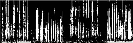
The binary mask got from SVM, as an example shown in Figure 2, can be treated as a two dimensional image. The image's height is the number of the channels of Gammatone Bank, and the image’s width is the number of the speech frames. The foreground (white blocks) in Figure 2 indicates the speech region, and the background (black blocks) indicates the noise region which should be filtered. We can see many isolated and unconnected white or black blocks in Figure 2. These isolated and unconnected blocks on a binary mask can be considered as the classification error. We, firstly, tried to use Connected Component Labeling and Hole Hilling to fix the problem.

Connected Component Labeling is an algorithm to label the unconnected component in image processing. Commonly used are 4-connected and 8-connected. Those pixels which are connected horizontally or vertically are considered to be the same object in 4-connected,and those pixels which are connected horizontally, vertically, or diagonally are considered to be the same object in 8-connected. 4-connected is used in our experiment.
The procedure is as presented in Figure 3. First, label each foreground pixels sequentially. Second, scan and change label from top left to bottom right. If the label of the current pixel is larger than the labels of upper pixel or left pixel, change it to the smallest label number. Again, scan and change label from bottom right to top left. The scan and change procedure will be repeated until all neighboring foregrounds have the same label. At last, we got the area of each connected foreground (speech) objects. Those isolated small area less than 2 points will be reclassified as background (noise).

For the holes on the foreground (speech), we use Hole Filling. Scanning from top left to bottom right, if one background pixel is surrounded by at least 3 pixels in 4 neighbors, we change the background pixel to foreground pixel. Only one scan is done. The binary mask after applying Connected Component Labeling and Hole Filling on Figure 2 is shown in Figure 4.
3.2 Morphology
Morphology is a popular algorithm in image processing to make the contour of objects smooth. It is used on our estimated binary mask to smooth the spectrogram. We applied one time Erosion and Dilation on the mask. Firstly, a foreground pixel is changed to background if it has a background pixel as a 4-neighbor. This procedure is called Erosion. Then, in Dilation, a background pixel is changed to foreground if it has a foreground pixel as a 4- neighbor.
4 Experiments
The clean speech corpus we used in our experiments is extracted from MAT-160 database recorded by the Association for Computational Linguistics and Chinese Language Processing (ACLCLP). It is divided into training set and testing set. 30 sentences recorded by 15 males and 15 females are used as training set. The total length is 140 seconds. 4 sentences recorded by 2 males and 2 females are used as testing set. The total length is 15 seconds. Five kinds of noise with different frequency characteristics are used. They are machine noise (in high band), siren noise (in medium band), babble noise (in wideband), white noise (in wideband) and factory noise (in low band). The first three kinds of noise with increasing energy level and total length of 140 seconds are used in training and separately added into clean testing speech as matched noise mixture, and the last two kinds are added into clean testing speech as unmatched noise mixture.
4.1 Signal-to-Noise Ratio
MFCCs and pitch are used as features of SVM to determine the binary mask to classify speech units and noise units. The experimental parameters are shown in Table 1.

Different measures are used to evaluate the experimental results. First, on signal level, we use Signal-to-Noise Ratio (SNR) to evaluate. Then, by comparing the ideal binary mask and the mask from our method, several measures are used including HIT-FA Rate (HIT rate minus False Alarm rate) [13,14], which is the difference between Hit Rate (Hit) and False Alarm rates (FA), True Rejection Rate (TRR), True-Acceptance Rate (TAR), Filtering Rate (FR) and Distortion Rate (DR).
First, we evaluate the classification performance of SVM alone. To do this, the post-processing (Connected Component Labeling, Hole Filling, and Morphology) on binary mask is not added in the experiments of 4.1 and 4.2.
The input sound mixtures with signal to matched noise or unmatched noise ratio of -3dB and 0dB are used in our experiment. After our speech segregation system, speech and noise are separated and the output SNRs are shown in Table 2.

As shown in Table 2, in matched noise condition, the -3dB mixture can improve to the average 7.33dB, and the 0dB mixture can improve to the average 9.35dB. In unmatched noise condition, the -3dB mixture can improve to the average 4.37dB, and the 0dB mixture can improve to the average 5.73dB.
4.2 True Rejection Rate and True Acceptance Rate
To test the classification performance of SVM, two experiments are set. The input of the first experiment is noise alone and we detect its True Rejection Rate (TRR). The input of the second experiment is clean speech and we detect its True Acceptance Rate (TAR). The TRR is the percentage of noise units a system correctly reject and the TAR is the percentage of speech units a system correctly verifies. In ideal cases, supposedly, we will get 100% TRR and TAR for noise (the first experiment) and clean speech (the second experiment) conditions.
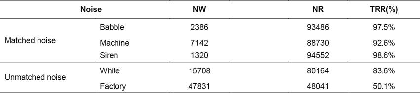
Table 3 present the TRR results of the matched or unmatched noise. NR is the number of correctly classified noise units (reject), and NW is the number of misclassified noise units (false alarm). SR is the number of correctly classified speech units (hit), and SW is the number of misclassified speech units (miss). As Shown in Table 3, obviously, it is more difficult to filter out noise correctly when the noise is unmatched (untrained). The result of factory noise, which distributes in low band and is difficult to distinguish with speech, is the worst.
Then, we input clean male (7.5 second long, the two male testing sentences) and clean female speech (7.5 second long, the two female testing sentences) separately. The result of TARs is shown in Table 4. The TAR is higher in female speech.

4.3 HIT-FA, Filtering Rate and Distortion Rate
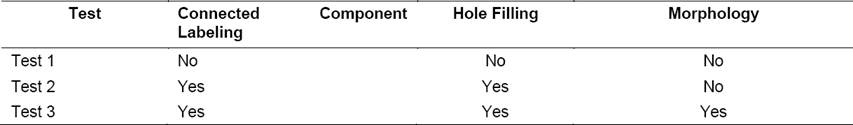
To further evaluate the performance of Connected Component Labeling, Hole Filling, and Morphology, we design three tests as in Table 5 and compare their results. Test 1 uses our system without Connected Component Labeling, Hole Filling, and Morphology. Test 2 uses Connected Component Labeling and Hole Filling only, and Test 3 uses all of the three.
Table 5 Three Tests to Evaluate the Performance of Connected Component Labeling, Hole Filling, and Morphology
Several measures are used, including HIT-FA, FR and DR. HIT-FA is the difference between HIT and FA and is useful in predicting the intelligibility of speech synthesized using estimated binary masks [13][14]. The HIT, FA, FR, and DR are defined as:
 (1)
(1)
 (2)
(2)
 (3)
(3)
 (4)
(4)
Higher FR and lower DR are desired for speech segregation.
To calculate these measures, we need to compare our estimated binary mask with ideal binary mask. In our experiment, ideal binary mask is defined as:
If both noise and speech energy are very small ( < 0.01), the T-F unit will be ignored and not put into calculation.
Else if speech energy > 0.5 * noise energy, the T-F unit is labeled as speech.
Else if speech energy ≦ 0.5 * noise energy, the T-F unit is labeled as noise.
An example resulting ideal binary mask is as shown in Figure 5. Blue area is labeled as speech and red area is labeled as noise. Black area are units with very small energy and can be ignored.

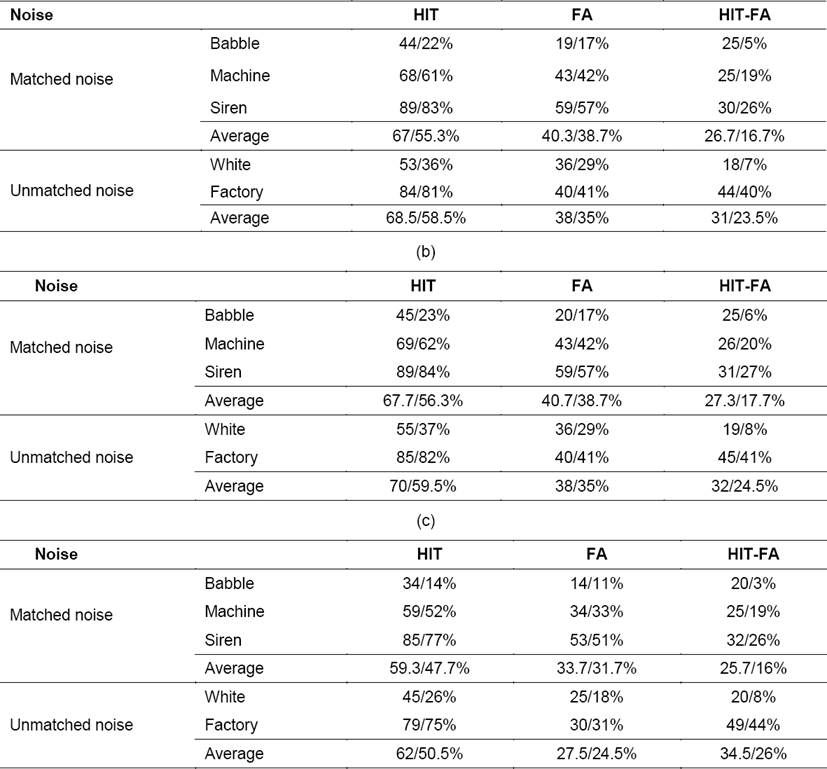
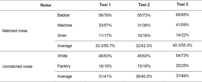
Table 6 is the result of HIT, FA, and FIT-FA of 0dB/-3dB mixture. The average unmatched noise HIT-FA of Test 3 is the highest, while the average matched noise HIT-FA of Test 2 is the highest. Table 7 and 8 show the FR and DR results of 0dB/-3dB mixture. Comparing the results shown in Table 7 and Table 8, Test 3 has higher FR and Test 2 using Connected Component Labeling and Hole Filling only has lower DR. That is, although Morphology can increase FR, it also increases DR.

The T-F units of -3 dB mixture with matched babble noise and unmatched white noise, the T-F results of Test 2, Test 3, and clean speech are shown in Figures 6 and 7. The waveforms of mixture, Test 3, and clean speech are also shown. Comparing our results with the sound mixtures, our method can successfully segregate speech and improve the speech quality.
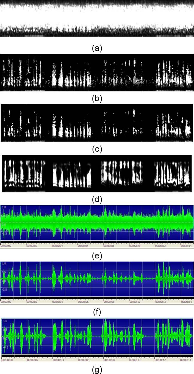
Fig. 6 T-F units of (a) -3 dB mixture with babble noise (b) Test 2 (c) Test 3 (d) clean speech. Waveforms of (e) -3 dB mixture with babble noise (f) Test 3 (g) clean speech

5 Conclusions
This paper proposes SVM classification and post-processing including Component Labeling, Hole Filling, and Morphology on CASA mask for speech segregation. By observing the results of different measures, T-F units, and waveforms, our method separates speech from background noise effectively.

