1 Introduction

Shallow parsing, or arbitrary phrase chunking is a well-known sequential tagging (more specifically a bracketing) problem. The CoNLL-2000 dataset [⁷] is the de facto standard dataset for measuring tagger performance in chunking for English. The current state-of-the-art method Gut, Besser, Chunker [²] achieves the F-score of 95.06% (96.49% for NPs). It is based on CRFsuite [⁵], a simple linear-chain conditional random field (CRF) tagger¹ and an improved version of the lexicalization of the previous state-of-the-art tagger, SS05 [⁶] (94.01% and 95.23% for NPs), which contains a lexicalization method invented by Molina and Pla [⁴] in conjunction with voting between different representations using HMM taggers (with only POS-tag as input).

It is notable that all the aforementioned methods use simple taggers with smart transformation of the input and output before and after tagging. Without this type of transformation even the most sophisticated tagger, which uses a bidirectional LSTM-CRF model [¹] only achieves 94.46 % F-score.

Indig and Endrédy questioned the methodology behind SS05 and compared different taggers on different levels of lexicalization with different voting schemes [²]. The authors could not reproduce the previous results due to the many programming errors discovered in the original code. But as a result of their thorough measurements they concluded that majority voting did not add much to the performance, therefore there is no real difference between the different representations and CRFsuite is the best performing tagger among the ones they compared. They also raised a question that all previous papers had left unanswered: ‘How does the tagger maintain well-formedness of tags?’².

However, the authors did not state anything about the lexicalization threshold³, which we investigate in this paper. We use their mild lexicalization with the CRFsuite tagger to find out the actual optimal values and to make statements about the stability of the method. We evaluate all five previous representations, even though it was shown that IOBES has superior performance to the other four [²].

We also present two methods (see Section 3 and 4) that may improve the accuracy of a tagger for a given test set. In the first method we adapt the lexicalization of the training set by using the input data from the test set. In the second method we use the uniform shape of the underlying Zipfian distributions of the development and test sets to get better parameter values automatically. We think that these two methods can be utilized for other tasks like POS tagging and NER as well, as word frequency is naturally available in all tasks and languages. In this paper we evaluate the two methods on English phrase chunking only. The following section covers the details needed to know on the topic.

2 Chunking, Representation of Chunks

Chunking is in fact a labeled bracketing problem translated into sequential tagging (B=[, E=], I=inside, O=outside, S=[]). They represent one level (labeled) bracketing that corresponds to the subtree of the parse tree of the sentence that contains the bracketed phrase. However, chunks can be assigned to tokens without real parsing, which would require more computational effort – and a full-fledged accurate parser that many languages still lacks – than sequential tagging. Using the same tagger framework one can solve tasks including but not limited to Part-of-Speech (POS) tagging and Named-entity recognition (NER). The aforementioned problems has an off-the-shelf solution as well for most of the languages which can be used for chunking to handle the lack of a real parser. Traditionally, also speed-up can be achieved by using tags that represent the position of a token in the sequence of bracketed entities, where each bracketed chunk can span multiple tokens similar to the representation of elements used in Named-entity recognition.

To lessen the number of classes and make the whole process even faster, there are representations of these brackets that omit some of the redundant classes which can be deduced automatically by the sequence of chunks (assuming well-formedness). In some cases this process makes the whole representation implicit (see IOX1 variants over IOX2 variants). To indicate a definite status of a token the following labels can be defined: beginning (B), inside (I), end (E), outside(O) of the sought phrases if there is such token. To be precise, one-token-long sequences must be indicated with a separate chunk type which is often denoted by single (S) or one-token-long (1). Each of the aforementioned tags except the O tag has an additional type or label when multiple type of chunks are sought. The reader may notice that using all of these indications, especially in conjunction with the chunk type labeling system are highly redundant. This gave rise to different representations with less number of chunk tags (see Table 1).

Table 1 Multiple IOB representations: An example sentence from the test set represented with five different IOB label sets 

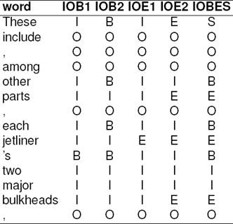
In addition to the numerous possible representations, one can find the following equivalent variants of the ‘full’ label set in the literature: the BILOU format⁴ (B=B, I=I, L=E, O=O, U=S) or the bracket variant ([=B, I=I, ]=E, O=O, []=S) which are equivalent to SBIEO⁵ or in a more conventional name, IOBES representation. We use the latter naming in this paper. The bracket variant in the untyped form is also called Open-Close notation (O+C or OC for short), but in this case the representation is very fragile and sensitive to the positioning of the tags as one mistake can destroy well-formedness.

The representations that use less tags still maintaining all information have two main types: the implicit (IOX1) and explicit (IOX2) variants, where X denotes the other important distinguishing feature: the omission of the beginning or the end tags as one of them is considered redundant. When only begin tags are used, one can choose from IOB1 or IOB2 tagsets and when only the end tags are in use there are the IOE1 and IOE2 representations.

In the implicit representation when two subse-quent chunks of the same type are found, one of the chunks is modified. In the IOB1 case the beginning I-tag of the second chunk is substituted with a B-tag of the same chunk type, and in the IOE1 case the ending I-tag of the first chunk is substituted with an E-tag of the same chunk type. Thus all the redundant tags are omitted (including S). The IOB2 variant is also referred to as BIO or IOB format or CoNLL format.

Note that without the chunktypes using the implicit variant of labeling, subsequent chunks of the same type can not be distinguished from each other. Therefore these versions are inferior to the others. Also in the untyped case, there is the prefixless notation where only chunk types are kept. And the Inside-Outside (IO) notation, where only the I and O labels are in use. In these two inferior variants, one can not distinguish consecutive chunks of the same type but they are useful for searching such patterns, because they are very simple and therefore fast.

One can see that the conversion between these representations is not trivial, but the Stanford CoreNLP’s IOBUtils [³] has the proper converter available to reliably convert between them and can also fix well-formedness issues (which feature we used in our measurements before the evaluation). These representations are traditionally handled uniformly, but we show how differently they behave⁶. For more information on the IOB representation see [⁸].

2.1 Lexicalization

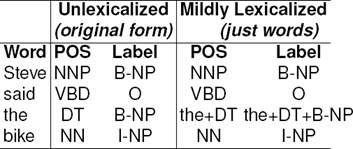
The lexicalization invented by Molina and Pla [⁴] is thoroughly investigated by Indig and Endrédy [²] and they present a mildly lexicalized variant (see Table 2) of the method that has superior performance. We use this variant in our measurements with different lexicalization thresholds. However, we are aware of the problem arising when using low thresholds that produce many labels and therefore make most of the taggers exponentially slow. Also we note that the number of invalid sequences grows with the number of classes as the taggers are not aware of well-formedness. The latter problem can be overcome by using a proper IOB converter which can also fix well-formedness issues (see Section 2 for details).

Table 2 Mild lexicalization: only IOB labels of the words above a given frequency threshold are augmented with the word and with its POS tag, otherwise the fields are left untouched. We use ‘+’ as separator because it is easier to parse than the originally used ‘-’ symbol 

The main motivation of the approach of Indig and Endrédy [²] was to reduce the number of labels because for agglutinative languages the original method is not feasible due to the high number of tags even without any lexicalization. But we also remark that this problem also exists with low thresholds used during lexicalization. Hypothetically, if we would lexicalize all vocabulary words, the whole problem could be reduced into a POS-tagging problem, with some extra tags added to represent the bracketing, so a totally different approach would be needed to maintain feasible training time.

The other problem with lexicalization is the difference between the test and development sets.

The development set has similar properties as the training set that it is stripped from, but in real life the test set is from another corpus with different frequency distribution of word forms. We also investigate whether (a) using frequent words from the test set for lexicalizing the training set and (b) transforming of the optimal threshold obtained on the development set to the test set yields better results and therefore makes the whole method more stable across different test sets.

3 Method

We separated a development set from the CoNLL-2000 training set by using every 10th sentence as it was used in the aforementioned papers. We used mild lexicalization and the CRFsuite tagger. For each of the five representations we applied training and test runs for the development and test sets with different lexicalization levels to see which threshold yields the optimal results.

As the size of the three sets differs⁷, we chose 10 as the lower bound and incremented the threshold by one till no words were left. The resulting word sets were used for lexicalization⁸. We lexicalized the three sets according to each lexicalization level conforming to the two lexicalization sources and tagged both the development and the test set yielding four tagging results per lexicalization level per representation⁹. The resulting tagged sets were then delexicalized and the well-formedness of tag sequences was fixed with IOBTools converter of CoreNLP [³] before evaluation. The gold standard annotation is only revealed in the evaluation step until then it was treated as non-existent as is for real life data, where the whole evaluation step is omited because there is no gold standard annotation for the tested set at all.

In order to determine the effect of our methods (see results in Table 3 and 4), we explored the resulting scores and searched for the best F-score achieved in the development phase to set the according lexicalization level for the measurements afterwards in the test phase. We distinguished two lexicalization sources (the test and the development set) that could be combined¹⁰ with the actual set to be tagged. Due to the difference of the development set and the prospective test set, we also measured the effect of the transformation of the lexicalization level – which was the best in the development phase – to accommodate the threshold to the lexicalization results of the test set in order to improve the results (see Table 4). The details of the transformation algorithm are presented in the next section.

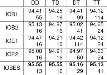
Table 3 Maximal scores on different setups (best lexicalization levels) [The lexicalization threshold is indicated below the score. Each representation has its maxima on different level, but around 16. (See Section 3 for column names)] 

Table 4 The final scores for the test set (with fixed lexicalization levels) 

4 Lexicalization Level Transformation

5 Results

Both the development and the test set have a Zipfian distribution underlying, but with different characteristics due to their different size and domain. We should find the appropriate slope for the tangent of the optimal threshold level on the Zipfian curve of the development set (using the two neighboring points of the curve). Using this slope, we can apply linear optimization to find the tangent with the same slope (denoted with a) on the test set’s Zipfian using the following formula: min_x,y (ax + y). The algorithm should return with the corresponding position of the curve for the test sets Zipfian yielding a more optimal lexicalization level that results from the invariant properties of the two Zipf curves (see Figure 1).

Fig. 1 Zipfian distribution of the development and test sets. The tangent of the curve corresponding to the lexicalization level producing the maximum score on the development set is transformed to the test set by linear optimization 

6 Lexicalization Thresholds for other Representations

For each lexicalization level we created the following test sets with their corresponding training sets: the development set lexicalized with the words yield from the development set (DD) to set the fixed lexicalization level for the measurements afterwards on the test set lexicalized with the words yield from the development set (TD) to determine the final F-score (see Table 3).

For comparison we also checked the same lexicalization threshold on the results of the test set lexicalized with the words yield from the test set (TT) and we also used a trasformed lexicalization level (Tr prefix) to see the improvement.

We does not reveal the gold standard annotation of the test set until the final evaluation part, so both presented methods (Section 3 and 4) can be used in real life for any test set with or without gold standard data.

In case of Section 3 the optimal parameters (threshold) are set previously on the development set therefore we do not train on (the gold standard annotation of) test set.

Independently, by transforming ‘blindly’ the optimal threshold gained from the development set to the test using the two Zipfians (Section 4) we do not utilize (the gold standard annotation of) the test set just the frequency distribution – which is available naturally – for the parameter adjustment.

On Figure 2 the best F-scores come from lower threshold levels. One can see a monotonic increase almost until the lowest lexicalization levels (60 ← 150). We can conclude that the IOBES variant has clear advantage over the other representations (about 1%) and the explicit (IOX2) variants beat the implicit (IOX1) variants (about 0.5%).

Fig. 2 Lexicalization thresholds for IOBES. (The other representations are similar. See Section 6) 

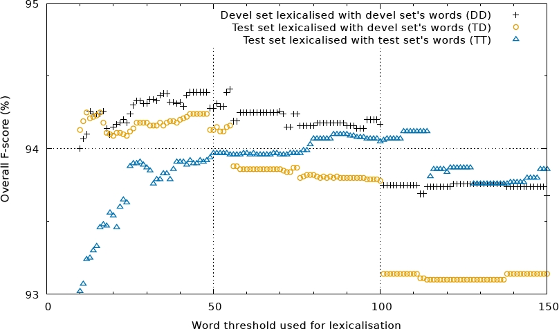
Fig. 3 Multiple lexicalization thresholds evaluated for IOB1 representation. Till about 50 the lexicalization with the test set’s words are clearly better. There is also a significant decrease after reaching the maxima around 16 

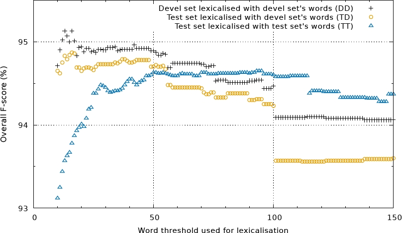
Fig. 4 Multiple lexicalization thresholds evaluated for IOB2 representation. Till about 50 the lexicalization with the test set’s words are clearly better. There is also a significant decrease after reaching the maxima around 16 

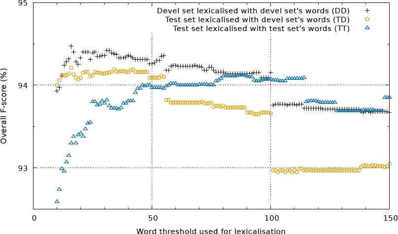
Fig. 5 Multiple lexicalization thresholds evaluated for IOE1 representation. Till about 50 the lexicalization with the test set’s words are clearly better. There is also a significant decrease after reaching the maxima around 16 

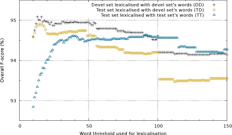
Fig. 6 Multiple lexicalization thresholds evaluated for IOE2 representation. Till about 50 the lexicalization with the test set’s words are clearly better. There is also a significant decrease after reaching the maxima around 16 

Until a threshold value of about 50, lexicalization with words of the test set is clearly better. There is a significant decrease after reaching the maximum around 16. On the right side of Figure 2, one can observe the biggest difference between the different lexicalization sources. The advantage of using the words from the test set is due to the fact that tokens with medium frequency are different from text to text.

Table 3 (training, development phase) contains the quantitative analysis of the different lexicalization models along with lexicalization thresholds that belong to the maxima¹¹.

One can see that most of the lexicalization levels that belong to the best F-scores (%) are below 50, which was tested by Shen and Sarkar [⁶] and Indig and Endrédy [²].

We can conclude that each lexicalization level behaves similarly regardless of the tested set, but the behavior of the two lexicalization models are quite different. In the development phase the best F-score (optimal upper bound) is achieved with the development set as lexicalization source. We used these lexicalization levels in Table 4 in the testing phase.

In Table 4 (testing phase with the predetermined lexicalization level) one can see that the best scores were achieved by using the words from the development set, but the transformation has improved the results of the raw mapping of the levels. The first column contains the maxima of the development set, the second and third column contains the raw mapping of the lexicalization level to the test set with the two lexicalization sources, the fourth column contains the transformed (Tr) values and scores, which are better than the raw scores (third column), but worse than the F-scores in the second column.

The final scores compared with the previous results are shown in Table 5 concluding that with a lower threshold we could gain 0.5% over the previous results on arbitrary phrase chunking.

Table 5 Summary of final F-scores, which out-performed the previous state-of-the-art results (+0.5% improvement) 

7 Conclusion and Future Work

We have presented a thorough analysis of different lexicalization levels with the current state-of-the-art method for arbitrary phrase chunking. Our detailed analysis revealed that the lexicalization level of 50, which was used in the previous state-of-the-art method was not the best choice. We could gain 0.5% after setting this threshold to 13. This leads to the conclusion that using this method for chunking is more similar to POS-tagging than to named-entity recognition and may be done simultaneously in the future.

We introduced a novel method that can be used to transform the parameters gained on the development set to the test set taking advantage of the invariant properties of the similarity of the two frequency distributions – which are naturally available – in order to have better and possibly more stable results. Using this transformation we could improve the results of the tagging near to the global optima of the underlying method, but could not beat the result of TD. However, we think lexicalization level transforming relevant for other tasks that benefit from finding frequency cut-offs across corpora.

Due to the fact that frequency distributions do not behave like normal functions because of the individual differences in the data, our linear optimisation method did not achieve the best F-scores. A higher level approximation that takes this fact into account better and uses more global information could make this method applicable.

For English the chunking task can be considered solved as nowadays there are many good-performing parser for English, but for other languages (that lack good parsers) the CoNLL-2000 dataset could be a good benchmark and our method may improve results for those languages or other tasks as well. Our software is available at: https://github.com/ppke-nlpg/less-is-more.