


 nova página do texto(beta)
 Inglês (pdf)
 Artigo em XML
 Referências do artigo
 Enviar este artigo por email
 Citado por SciELO
  Similares em
SciELO
Similares em
SciELO 
 Permalink
1 Introduction
The great advances in the field of neuron tracing have made possible a high availability of data in the Internet, which encourages the realization of automatic classifications [21, 3]. Note that although the issue of classifying neurons had its beginnings since the emergence of the neuroscience as a scientific discipline, manual classification is a slow and tedious task for human analysts, and this fact determines the existence of an increasing interest in the use of machine learning techniques for this application [2]. It is worth to mention that manual classification is also subjected to inter- and intra-analyst variability due to the subjectivity inherent to this process. Major efforts have been made in terms of automatic classification of neurons, but most of them have been done by using unsupervised techniques [14, 19]. These have been exploratory techniques aimed at discovering new types of cells or to confirm some known hypotheses about the neurons. Although useful, these classification systems are hampered by at least two deficiencies. First, a distinctive feature can be shared by several cell types. Second, one discriminative feature for certain neuronal types may be irrelevant and highly variable for other types. It is therefore necessary to find new descriptors having discriminative properties in regard of neuron classes, in order to improve the automatic classification.
Today neural structures such as the axon and the dendrites remain the cornerstone in the analysis of neural development; pathology; computation and connections between neurons [21]. Neuron classification, however, has also been treated as a multimodal problem in which in addition to the morphological features, biochemical and electrophysiological features are also employed [13]. There are several software that perform morphometric analysis [22, 17, 7, 1]. The morphometric features are oriented mainly to the density of the branches of neuronal trees, the size of the roads and the relationship between their thickness, tortuosity, angles at bifurcations, volume and area, among others. One of the most commonly used ways to quantify neurons is the Sholl analysis, to which several modifications have already been made [10, 11]. In order to characterize neurons and find common rules in the geometry of the dendrites, a study related with the angles formed by its branches has been carried out in [18]. Another way to represent the structure of neuronal trees is proposed in [12], where bifurcations are encoded as strings.
In this study we focus the attention in the use of morphological features for supervised classification, which has been less treated and has shown better results than unsupervised techniques [14, 23]. In this case, a priori information which is used in unsupervised algorithms only to validate the classification process, allowed us to build our models. This paper presents a comparative analysis among different supervised learning techniques, oriented to the classification of reconstructed neurons using morphological features.
2 Materials and Methods
The data used for classification were extracted from the NeuroMorpho.Org website, which contains a large number of neuronal reconstructions from different species, brain regions and laboratories [15], freely downloadable. Neural reconstructions used in our research came from [14], where the procedure for the used neuron reconstruction process is explained in detail. The neurons reconstructed there belong to laboratory rats. This data set is composed of 318 traced neurons, classified by human experts in 192 interneurons and 126 pyramidal cells. The features were computed from arbor reconstruction files in the standard SWC file format. From each of these cells a set of morphometric features were computed to be used later in the classification process. The way of representing the neurons is by means of a graph, where their branching structures are represented by the directed adjacency matrix. A tree is composed by a set of labelled nodes connected by edges, these edges are also called compartments and they have an associated diameter. Only the compartments associated to a specific feature are to be taken into account, the rest being discarded.
The first data set (called LM) is composed by features extracted using the L-Measure software, which provides 43 morphological features. Each of these features is associated with 7 parameters [22], as shown in Table 1. In many cases, some of these 7 parameters are meaningless, therefore it is necessary to preprocess the data set. The second data set (called NF) is composed by new features proposed in this research which are shown in Table 2.

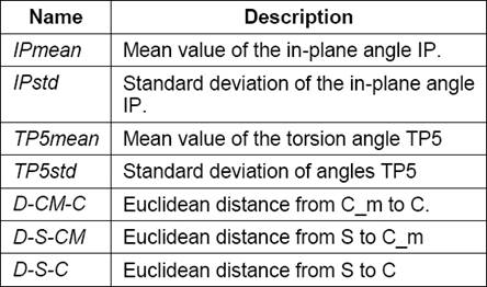
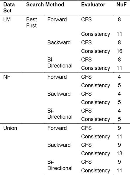
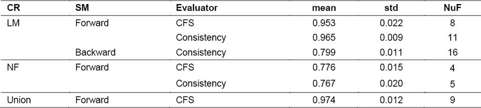
Table 3 Results after applying feature selection techniques for each dataset, showing the number of feature (NuF) obtained
The 3rd data set is simply the union of the two previous ones (called Union), and it was created in order to determine if the incorporation of the proposed features can improve the performance of classifiers. Three matrices were then formed, having 318 rows and a number of columns equal to the number of features used. Some feature selection techniques were used to reduce the cardinality of the data sets. This was made in order to comply with the recommendations made in [9], about having an appropriate relationship between the numbers of cases and features to prevent overfitting of the classification algorithms, This procedure tends also to improve the performance of classifiers.
2.1 Feature Selection
A selection was made of a subset of the features included in the original set, with the purpose of obtaining maximum performance with minimum effort. All feature selection algorithm consists of two basic components: evaluation function and search method. As search method was used Best First, with three alternatives: Forward, Backward and Bi-Directional. In the case of the evaluation function, the methods used were Correlation-based Feature Selection (CFS) and Consistency-based Subset Evaluation. The CFS evaluation function tends to produce subsets containing features that are highly correlated with the class and uncorrelated between them [16]. In the case of Consistency, it is characterized by having a strong dependence on the training set, trying to remove the minimum subset that satisfies an acceptable rate of inconsistency, usually set by the user.
2.2 Neuronal Classification
The classification process had two purposes: to determine whether using the new proposed features improved the quality of classification and to compare the performance of several classifiers. The metric selected to quantify the performance of classifiers was the AUC or area under the ROC (receiver operating characteristic) curve. As methods of machine learning classifiers were used Logistic Regression (LR), KNN, Random Forest (RF), C4.5 and Naive Bayes (NB) [8]. Both feature selection techniques and classification algorithms were applied using the widely known open-source data mining software tools named WEKA [6]. The parameters of the classifiers were those who come by default in WEKA. For KNN we decided to use k = 3, since this value led to the best result obtained during the experiments.
The R software was used, specifically the SCMAMP package, in order to apply statistical tests [4]. We applied 5x2cv as described in [5] as well as the Friedman test, to find out if there were significant differences between some of the classifiers analyzed. In the case where such differences were found, the Finnes post hoc test was applied, which is considered generally a good choice because of its simplicity and power.
2.3 New Proposed Features
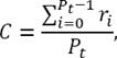
The first feature implemented was the in-plane angle (IP i ). It is computed using three points of the neuron, as it is shown in equation 1. Figure 1 shows the vectors to compute the angles in the neurons:
 (1)
(1)
where


Notice that the point P i has the coordinates (X i Y i Z i ) in a three dimensional space and in this analysis it is represented by a position vector traced from the coordinate axes’ origin up to the point itself. The number of IP i calculated for the whole neuron is computed by equation 2, where Pt is a total of nodes and Pter is a number terminal points. Notice that it is necessary also to subtract one, because the initial point is not counted:
 (2)
(2)
Another feature implemented was the torsion angle. It is composed of the angle between two consecutive planes whose pivot point is P i .
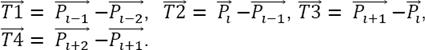
Then using the procedure described above for the vectors associated to points P
i−1
and P
i−2
, we defined  and analogously from the vectors associated to P
i+1
and P
i+2
is defined
and analogously from the vectors associated to P
i+1
and P
i+2
is defined 
The orthogonal vectors to the two planes containing the vectors ,  and
and  , were obtained using the vector cross product and then the angle between these vectors which corresponds to the rotation between the two planes considered is calculated as shown in equation 3:
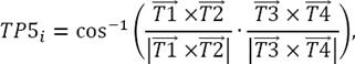 (3)
(3)
where
The number of torsion angles calculated for the whole neuron is computed by equation 4, where Pt is the total number of points (nodes) and Pter is the number of terminal points in the neuron:
 (4)
(4)
For the list obtained with TP5
i
, we compute global statistics like mean ( ) and standard deviation (𝜎). Notice that differently to what is proposed in [17], to compute the torsion angle we used here five points instead of four, as shown in Figure 1.
The features calculated afterwards are associated with the Euclidean distances in the three-dimensional space formed between three points. The first is the root of neuron tree (soma, S).
The second point is the centroid (C) of the tree, and the third is the center of mass (C m ). C is defined by equation 5. C m is computed using equation 6, where r i is the position vector (X i , Y i , Z i ) and V i is associated with the cylindrical volume formed between two consecutive nodes, which has its radius as prior information.
Its height (ℎ) is calculated as the distance between the two node points, as shown in equation 7. The description of the implemented features is shown in Table 2:
 (5)
(5)
 (6)
(6)
 (7)
(7)
Figure 2 and Figure 3 show examples of the classes of neurons that are being analyzed in this research. In these figures it is observed the graphical representation of some of the new features proposed, notice that the distances between the above mentioned node points are different.


3 Results and Discussion
Once the feature selection method is applied, new subsets of features are obtained, which coincide in many cases, as shown in Table 2.
In the case of the set LM and using the CFS evaluator, the same subset of features is obtained by the three search methods. The new subset contained 8 features. On the other hand, the selection using the Consistency evaluator led to different results when compared to the previous one. The Forward and Bi-Directional search strategies selected the same subset of 11 features and in the case of the Backward search method the subset had 16 features.
For the Union set, the results obtained using the Consistency evaluator were the same obtained for the LM subset, i.e. the feature selection method chose the same subset of features in the case of LM as well as in the case of Union. Something different happened with the CFS evaluator for the Union set where nine features were selected. Three of these 9 features selected belonged to the NF set, these were IPmean, D-S-Cm and TP5mean i.e. three out of the nine features contained in this set, were among the new features proposed.
In the case of NF with the CFS evaluator, there is a coincidence among the sets of features obtained for the cases of Forward, Backward and Bi-Directional, resulting in a total of four features. In the case of the Consistency evaluator, the resulting subset contained five features instead of 4.
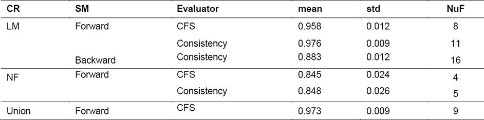
Table 4 shows the results of the LM classifier for the subsets of features obtained with different feature selection techniques. Given that in some cases the subsets match, the results of the classification were also the same. Hence only the results that were different are shown. For the first subset of features belonging to the set obtained from L-Measure, the highest value was 0.965, using the Consistency evaluator with 11 features. In the case of the second set of features (NF, proposed in this research) AUC values ranged between 0.76 and 0.77, demonstrating its discriminative power, however they did not reach the values achieved by the features from L-Measure.
In the case of the last set of features that is the union of the previous two sets, relatively higher values were obtained than those previously achieved independently when using features from L-Measure and the AUC for the new features attained the value 0.974, and this was the highest AUC performance for this classifier. It is pointed out that the subset obtained with Union had fewer features and better performance in the classification, making this subset more computationally efficient.
The Random Forest classifier performance is shown in Table 5. It is observed that there was a noticeable increase in AUC for the case of the new features proposed, because in the previous classifiers AUC were around 0.77 while now this value was raised up to 0.847. We also found for this classifier a higher AUC value of 0.976, which was reached with the LM set using the Consistency search strategy and 11 features. However, the Union set also had a good performance, demonstrating that the proposed new features together with those calculated with L-Measure are a good alternative for automatic classification of these classes of reconstructed neurons.
3.1 Comparison between Classifiers
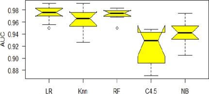
Taking into account that the best performances of the classifiers were observed for the Union set of features, this was used as a basis to determine whether there are significant differences between the performance of the five classifiers that were used in the experiments. Fig shows the distribution for each classifier of the calculated AUCs in each of the classification experiments.
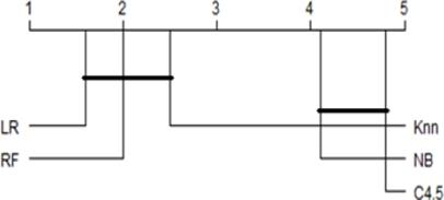
After applying the Friedman aligned rank test, the p value was less than 0.05, which means that there were significant differences between the classifiers used. To find out between which of these classifier existed significant differences, the Finnes post hoc test was applied, the results of which are shown in Figure 5. In this figure it is observed that there were neither significant differences between the classifiers forming the first group, LR, RF and KNN, nor differences between those forming the second group, e. g. C4.5 and NB, while there were significant differences between these two groups according to which the first group exhibited a better performance.
4 Conclusions
In this study, various methods to classify reconstructed (traced) neurons were compared, based on the extraction of morphological features by means of the L-Measure software and new features proposed by the authors. Feature selection methods were employed to establish an appropriate relationship between the number of cases and the number of features in order to avoid overfitting of the classification algorithms.
The data used were downloaded from the NeuroMorpho.org website, which offers the largest number of reconstructed neurons freely downloadable in the Internet. There were introduced eight new features with the purpose of increasing the discriminative power of the automatic classification algorithms. These features were based on the in-plane deviation and torsion angles in the neural tree as well as in the distance from S to Cm (D-S-Cm). The Union subset of features which contained the new features, showed in many cases an improvement of the classification performance. In addition, this subset had a lower number of features, which made it computationally less expensive. The statistical analysis showed that the best classifiers were LR, RF and KNN.

