1 Introduction

Since the most famous random graph model was proposed by Erdös and Rényi [¹], the complex network has attracted much attention in many fields of research, such as biology, physics, computer networks, the World Wide Web (WWW) [²], and so on. Network synchronization has obvious advantages, it has great application value in practice. Therefore, Atay et al. [³] studied synchronization of complex network when delays exist among the nodes; Motter et al. [⁴] studied the influence of coupling strength on the synchronizing ability of a complex network; Timme et al. [⁵] studied the web synchronization law of pulse-coupled dynamical systems; Checco et al. [⁶] studied the synchronization of random web. Lü et al. [⁷] constructed general complex dynamical networks and studied the synchronization; Lu and Chen [⁸] studied synchronization analysis of linearly coupled networks of discrete time systems; Han and Lu [⁹] studied the changes of synchronization ability of coupled networks from ring networks to chain networks; He and Yang [¹⁰] studied adaptive synchronization in nonlinearly coupled dynamical networks.

The analysis and control of complex behavior in complex networks, which consist of dynamical nodes, has become a point of great interest in recent studies, [¹¹, ¹², ¹³]. The complexity in networks comes from their structure and dynamics but also from their topology, which often axoects their function. Recurrent neural networks have been widely used in the fields of optimization, pattern recognition, signal processing and control systems, among others. They have to be designed in such a way that there is one equilibrium point that is globally asymptotically stable. In biological and artificial neural networks, time delays arise in the processing of information storage and transmission. Also, it is known that these delays can create oscillatory or even unstable trajectories. Trajectory tracking is a very interesting problem in the field of theory of systems control; it allows the implementation of important tasks for automatic control such as: high speed target recognition and tracking, real-time visual inspection, and recognition of context sensitive and moving scenes, among others.

The motivation in this paper lies in the complex network synchronization and chaos control importance. Network synchronization is one of the most practical and valuable issues. A synchronization of network means the situation in which the output of all nodes in the study of the complex network is consistent with any given external input signal under a certain condition. Numerical simulations are used to verify the effectiveness of the proposed techniques. We present the results of the design of a control law that guarantees the tracking of general complex dynamical networks.

2 Mathematical Models

2.1 General Complex Dynamical Network

Consider a network consisting of N linearly and diffusively coupled nodes, with each node being an n-dimensional dynamical system, described by

(1)

where x _i = (x _i1 , x _i2 , . . . , x _in ) ^T ∈ ℝ ⁿ are the state vectors of node i, f _i : ℝ ⁿ 7 ↦ ℝ ⁿ represents the self-dynamics of node i, constants c _ij > 0 are the coupling strengths between node i and node j, with i, j = 1, 2, . . . , N. Γ = (τij) ∈ ℝ ^n×n is a constant internal matrix that describes the way of linking the components in each pair of connected node vectors (x _j − x _i ): that is to say for some pairs (i, j) with 1 ≤ i, j ≤ n and τij ≠ 0 the two coupled nodes are linked through their ith and jth sub-state variables, respectively, while the coupling matrix A = (a _ij ) ∈ ℝ ^N×N denotes the coupling configuration of the entire network: that is to say if there is a connection between node i and node j(i ≠ j), then a _ij = a _ji = 1; otherwise a _ij = a _ji = 0.

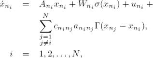
2.2 Recurrent Neural Network

Consider a recurrent neural network in the following form:

(2)

where xni = (xni, xni2,…,xnin) ^T ∈ ℝ ⁿ is the state vector of neural network i, Uni ∈ ℝ ⁿ is the input of neural network i, Ani = -λni I _n×n , i = 1, 2, . . . , N, is the state feedback matrix, with λni being a positive constant, Wni ∈ ℝ ^n×n is the connection weight matrix with i = 1, 2, . . . , N, and σ(·) ∈ ℝ ⁿ is a Lipschitz sigmoid vector function [¹⁴], [¹⁵], such that σ(xni ) = 0 only at xni = 0, with Lipschitz constant Lσi , i = 1, 2, . . . , N and neuron activation functions σ _i (·) = tanh(·), i = 1, 2, . . . , n.

3 Trajectory Tracking

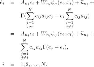
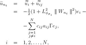
The objetive is to develop a control law such that the ith neural network (2) tracks to the trajectory of the ith dynamical system (1). We define the tracking error as e _i = x _ni − x _i , i = 1, 2, . . . , N whose time derivative is

(3)

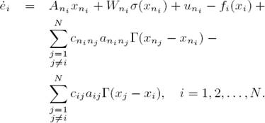
Substituting (1) and (2) in (3), we obtain

(4)

Adding and substracting Wni σ(x _i ), α _i (t), i = 1, 2, . . . , N, to (4), where α _i to be determined below, and taking into account that xni = e _i + x _i , i = 1, 2, . . . , N, then

(5)

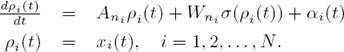
In order to guarantee that the ith neural network (2) tracks the ith reference trajectory (1), the following assumption has to be satisfied:

Assumption 1. There exist functions ρ _i (t) and α _i (t), i = 1, 2, . . . , N, such that

(6)

Let define

(7)

Considering (6) and (7), the equation (5) is reduced to

(8)

Rewriting the summations as

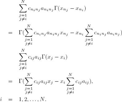(9)

also taking into account that cninj = c _ij and aninj = a _ij , then, using the equations above (8) becomes

(10)

It is clear that e _i = 0, i = 1, 2, . . . , N is an equilibrium point of (10), when , i = 1, 2, . . . , N. In this way, the tracking problem can be restated as a global asymptotic stabilization problem for system (10).

4 Tracking Error Stabilization and Control Design

In order to establish the convergence of (10) to ei = 0, i = 1, 2, . . . , N, which ensures the desired tracking, first, we propose the following candidate Lyapunov function

(11)

The time derivative of (11), along the trajectories of (10), is

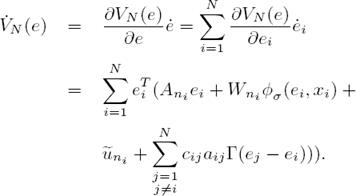(12)

Reformulating (12), we get

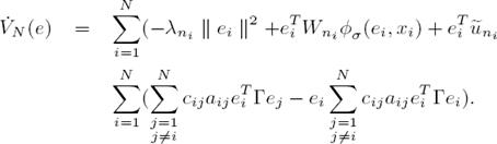(13)

Next, let consider the following inequality, proved in [¹⁶, ¹⁷]:

(14)

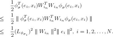
which holds for all matrices X, Y ∈ ℝ ^n×k and Λ ∈ ℝ ^n×n with Λ = Λ ^T > 0. Applying (14) with Λ = I _n×n to the term e _i ^T W _in φ _σ (e _i , x _i ), i = 1, 2, . . . , N we get

(15)

Then we have that, and taking into account that φ _σ is Lypchitz:

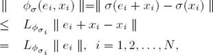(16)

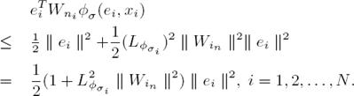
with Lipschitz constant . Applying (16) to 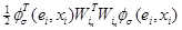we obtain

(17)

By simplifying (15), we obtain

(18)

Then we have that:

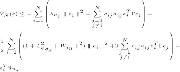(19)

We define e, i = 1, 2, . . . , N, then (19) becomes in

(20)

Now, we propose to use the following control law:

(21)

then for all e ≠ 0.

This means that the proposed control law (21) can globally and asymptotically stabilize the ith error system (10), thereby ensuring the tracking of (1) by (2). Finally, the control action driving the recurrent neural networks is given by

(22)

5 Simulations

In order to illustrate the applicability of the discussed results, we consider a dynamical network with just one Lorentz’s node and three identical Chen’s nodes. The single Lorentz´s system is described by

(23)

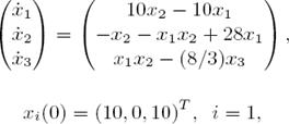
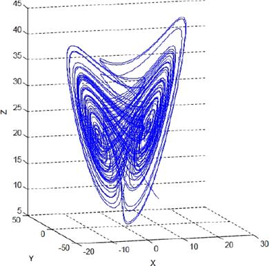
and the Chen’s oscillator is described by Eq. 24:

(24)

If the system parameters are selected as p ₁ = 35, p ₂ = 3, p ₃ = 28, then the Lorentz’s system and Chen’s system are shown in Fig. 1 and Fig.2 respectively. In this set of system parameters, one unstable equilibrium point of the oscillator (24) is x = (7 : 9373; 7 : 9373; 21)T .

Fig. 1 Sub-State of Lorentz’s attractor with initial condition X ₁(0) = (10, 0, 10) ^T  

Fig. 2 Sub-States of Chen’s attractor with initial condition X2;3;4(0) = (−10, 0, 37) ^T  

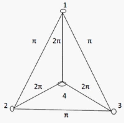
Suppose that each pair of two connected Lorentz and Chen’s oscillators are linked together through their identical sub-state variables, i.e., Γ = diag(1, 1, 1), and the coupling strengths are c ₁₂ = c ₂₁ = π, c ₁₃ = c ₃₁ = π, c ₂₃ = c ₃₂ = π, c ₁₄ = c ₄₁ = 2π, c ₂₄ = c ₄₂ = 2π, c ₃₄ = c ₄₃ = 2π. Fig. 3 visualizes this entire dynamical network:

Fig. 3 Structure of the network with each node being a Lorentz and Chen’s system 

The neural network was selected as

(25)

Theorem 1 For the unknown nonlinear sys-tem modeled by (1), the on-line learning law tr {W ^T W} = −e ^T W σ(x) and the control law (22) ensure the tracking of to the nonlinear reference model (2).

Remark 2 From (20) we have, ∀ e ≠ 0, ∀W, and therefore V is decreasing and bounded from below by V (0). Since , then we conclude that e, W ∈ L _1; this means that the weights remain bounded.

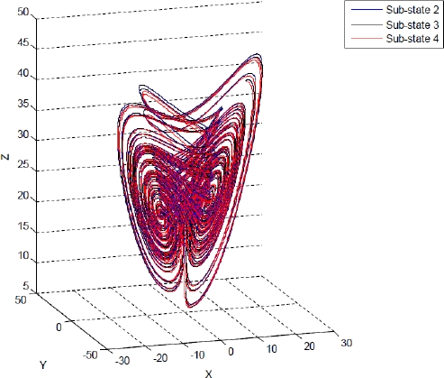
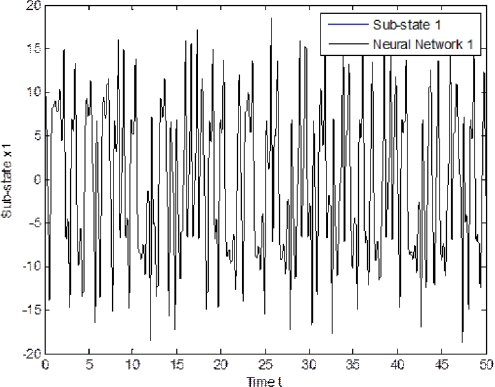
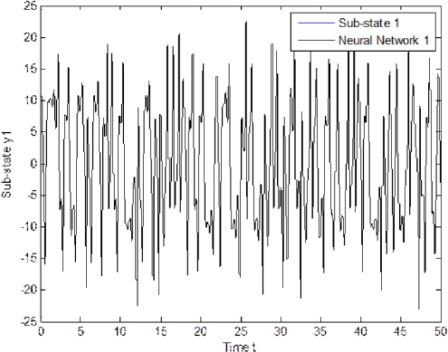
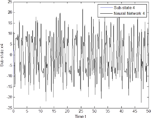
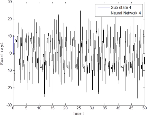
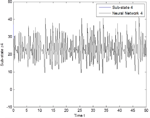
The experiment is performed as follows. Both systems, the recurrent neural network (2) and the dynamical networks (24) and (25), evolve independently; at that time, the proposed control law (23) is incepted. Simulation results are presented in Fig. 4 - Fig. 6 for sub-sates of node 1. As can be seen, tracking is successfully achieved and error is asymptotically stable, as it is shown in Fig. 7 -Fig. 9 for sub-states of node 4.

Fig. 4 Time evolution for sub-states 1 with initial state X _n1 (0) = (10, 0, 10) ^T  

Fig. 5 Time evolution for sub-states 1 with initial state X _n1 (0) = (10, 0, 10) ^T  

Fig. 6 Time evolution for sub-states 2 with initial state X _n1 (0) = (10, 0, 10) ^T  

Fig. 7 Time evolution for sub-states 4 with initial state X _n4 (0) = (20, 20, −10) ^T  

Fig. 8 Time evolution for sub-states 4 with initial state X _n4 (0) = (20, 20, −10) ^T  

Fig. 9 Time evolution for sub-states 4 with initial state X _n4 (0) = (20, 20, −10) ^T  

6 Conclusions

We have presented the controller design for trajectory tracking determined by a general complex dynamical network. This framework is based on dynamic recurrent neural networks and the methodology is based on Lyapunov theory. The proposed control is applied to a dynamical network with each node being a Lorenz and Chen’s dynamical system, respectively, being able to also stabilize in asymptotic form the tracking error between two systems. The results of the simulation shows clearly the desired tracking. In future work, we will consider the stochastic case for the complex dynamical network.