1 Introduction

Steam turbines play a dominant role in the generation of mains electrical supply and the prospects of improved designs resulting from greater understanding are good [¹]. The existence of the liquid phase in the low pressure (LP) steam turbines, formed by a polydispersed (different sizes) system of droplets, leads to loss of performance.

Additional energy losses, blade erosion and blade failures due to corrosion effects in the phase transition zone thus result in decreased turbine efficiency reliability [²]. This is attributed collectively to wetness losses, but the detailed mechanisms that give rise to these are insufficiently understood. In addition, the wetness loss is influenced by deposition rate, since it depends on the distribution of the total water content of the flow between fog drops and large drops (referred as coarse water) which are formed when deposited water is stripped from blade trailing edges.

A number of numerical studies, over the past several decades, have been directed toward modeling two-phase flow behavior of wet steam [³]. While Navier-Stokes solvers are needed to obtain accurate solutions for viscous flows in turbomachines, a fast Euler solver is still a desirable tool for routine applications particularly in problems, where viscous effects are confined to the walls regions. In this regard the numerical approach most often used has been the inviscid-time marching scheme.

McDonald [³] was the first investigator to use the time marching, Finite Volume Method (FVM). Denton [⁴] extended McDonald’s finite-volume method and has been used in inviscid viscous interaction programs for turbomachinery calculations. In these models the dispersed water phase can be handled via particle tracking along streamlines; this provides a wetness distribution (which is fundamental information for solving and minimizing the above wet steam effects in steam turbines) and hence mixture conditions for the subsequent single-phase inviscid flow calculation.

Young [⁵] reduced computational time and effort when he introduced a semi-analytical technique for investigating the thermal effects in wet-steam turbines, Ahmadi [⁶] simulated a two-dimensional inviscid transonic cascade flow using a cell-vertex finite volume space discretization method on unstructured triangular meshes. Qulan and co-workers in [²] proposed a numerical framework to study water drop erosion on turbine blades, it coupled fluid mechanics with solid mechanics.

In this work, inviscid flow is simulated by solving Euler equations on a purely triangular mesh using a time-marching solution method. The time dependent integral form of the equations is discretized in space using a cell-vertex FVM. Convergence acceleration is achieved by employing a polynomial smoothing. The governing equations, the discretization and the boundary conditions implementation are first presented. It is followed by the two-phase approach for modeling the interaction between the gas and liquid phases. The use of a two-phase approach has the potential for incorporating much more complex droplet models, since the two phases do not have to share the same velocity field.

2 Governing Equations and Discretization

Considering unsteady, inviscid two-dimensional compressible flow of a vapor carrying a population of droplets with no interphase slip, the continuity, momentum and energy equations, governing the unsteady two-dimensional flow of an inviscid fluid (known as the Euler equations) are written in conservative form in a Cartesian coordinate system [⁷] as follows:

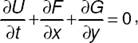(1)

where U is a state vector of dependent variables and F and G are the flux vectors in the x and y directions, and are given by:

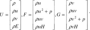(2)

Also it is needed the equation of state:

(3)

and for a polytropic process

(4)

When the solution of steady flows is of interest it is assumed that the flow takes place at constant stagnation enthalpy and the energy equation is written as:

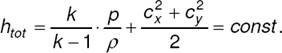(5)

This assumption is exact when the flow becomes steady, even in the presence of shock waves.

For the scheme to be effective the equations must be solved in the order: mass-pressure-momentum. The order in which the momentum equations are solved is not important. The procedure adopted is to update the density from the continuity equation at all grid points then update the pressure from the equation of state. Finally, the new pressures together with the old densities and velocities are used to update the x momentum and y momentum. The method is therefore explicit [⁸], in the sense that the new variables are not used in the time step in which they are calculated with the exception that the new pressure is used immediately it is available.

The boundary conditions applied at the downstream boundary are: a specified uniform static pressures and a condition of zero velocity gradient along the streamlines. At the upstream boundary the stagnation pressure and flow direction are specified.

A simple stability analysis has been developed for the scheme, and the maximum permissible time step can be calculated as:

(6)

A homogeneous dispersed two-phase flow exists, in case the dispersed phase is distributed homogeneous in the continuous phase. The dispersed two-phase flow with steam as continuous phase and water droplets as the dispersed water is the essential part of the investigations in the present work. The volume fraction αp is the ratio of the volume of the droplets to the total volume:

(7)

with Vp being the droplet volume.

The present model relies on a Lagrangian representation of the water droplet phase. The following describes how the Lagrangian tracking model was implemented for the cases of freshly nucleated and larger droplets. The motion model assumes the slip between the droplet and the surrounding gas.

This is a reasonable assumption considering that the radius of a freshly nucleated droplet may grow to a size in the range of 10^-7 m within the extent of the solution domain [⁹]. The method used in this work is based on the calculation of the path of several individual solid particles through the flow field. Each particle represents a sample of particles that follow an identical path. The motion of the tracked particles is taken to describe the average behavior of the discrete phase. While setting up the Lagrangian tracking and the deposition model described below, the following assumptions have been made according to Ahmadi in [⁶]:

We do consider, according to Ulrichs [¹⁰]:

Change of the continuous trajectory due to the effect of the discrete phase trajectories on the continuum (this is a condition for monitoring erosion).

We need to specify, according to Mashmoushy in [¹¹]:

The particles are injected and tracked through a network of flux-elements. The gas-phase equations are solved at the control-volume locations. When a particle is injected into the flow (for steady-state calculations) the particle is tracked until some fate is reached, such as impacting a wall, passing into a periodic boundary or exiting the flow domain. For a particular fate, a predetermined action is undertaken such as leaving the domain (outflow), translation and reinjection (periodic condition) and collection [¹²].

During a particle’s journey to a particular fate it will pass through a succession of flux-elements, and the inertia force of a particle in a gas flow is in equilibrium with all forces acting on the particle:

(8)

The forces F _i include the drag force, F _D (v - v _p ), and the force required to accelerate the fluid surrounding the particle with diameter D _p , mass m _p , density ρ _p . and velocity v _p . This model permits us to simulate a discrete second phase in a Lagrangian frame of reference, where the second phase consists of spherical particles dispersed in the continuous phase.

In what follows, all distances are non-dimensionalized (except droplet deposition rate) using an appropriate characteristic length and all flow variables are non-dimensionalized as follows:

(9)

A cell-vertex finite volume method is used to discretize the equations of motion, eq. (1), on a structured triangular mesh. The computational domain is divided into triangles, fixed in time, and the flow variables are stored at their vertices. For any node, the control volume (surface in 2D) is taken as the union of all triangles with a vertex at that node, i. e. the control volumes are overlapping.

The governing equations, eq. (1), are then integrated over each control volume Ω (surface in 2D) which is bounded by the surface δΩ (curve in 2D), and using Gauss theorem (Green’s theorem in 2D) one obtains:

(10)

The fluxes F and G along a particular edge of the control volume are numerically evaluated as the average of the nodal flux values at the ends of that edge. When the cell-vertex discretization scheme is applied to eq. (10), we get the following set of equations for each cell i:

(11)

where the summation is taken over all edges of cell i. S _i is the cell area, R _i is the solution vector, F _e and G _e are the components of the flux vector on edge e, and n _xe , n _ye are the components of the outward normal to edge e. when eq. (11) is written for all cells i, we get:

(12)

where Q (R _i ) represents the discrete approximation to the convective flux integral.

3 Computational Method

A two-dimensional wet steam flow is described by the system of Eulerian/Lagrangian equations in which the conservation equations of gas dynamics were solved in Eulerian formulation while the liquid phase was treated in Lagrangian coordinates. This model allows the droplet integration to be separated from the grid size, and gas phase time step, allowing for a coarser grid to be employed. Since each droplet size is integrated from its initial creation to a final fate, no special handling is required to account for movement through a wide range of size regimes.

Time marching methods are in principle the most flexible means of calculating blade-to-blade flows in turbomachinery since the same method can be used for subsonic, transonic and supersonic flows with automatic inclusion of time dependence. The basic principle of time marching is to start with a guess flow distribution and integrate the time dependent equations of motion forward with time until a steady-state solution is obtained.

The concept chosen was to use McDonald’s elemental control volume but with an H grid. The mesh is formed by a series of quasi-streamlines which are evenly spaced in the y direction and by pitchwise direction lines which need not be evenly spaced in x direction.

The quasi-streamlines upstream and downstream of the cascade are chosen to be roughly in line with the flow inlet and outlet directions but these lines do not control the flow direction. The outlet flow direction is obtained as part of the calculation being determined by the periodicity condition behind the trailing edge. Periodic boundaries are treated in the same way as solid boundaries but after each time step the properties at corresponding points are averaged.

The computational code was structured in three parts: the first program produces the two dimensional finite mesh system of turbine cascade and the input data are: profile length, staple angle and number of original profile coordinates.

The second program calculates the density and momentum distributions of 2-dimensional transonic potential flow by time step method at turbine cascade, the input data are: x and y - axial mesh coordinates, upstream velocity, upstream pressure, downstream pressure, upstream density, upstream flow angle, isentropic exponent, efficiency of turbine cascade, time segment; the third program obtains the drop trajectories and humidity distributions of two dimensional turbine cascade.

Relevant input data are: radius of particle, density of particle, dynamic viscosity and upstream humidity.

4 Results

A series of results is presented, which includes the simulations carried out with the stator configuration. At inlet, the relative flow angle varies from 90° to 120°, and the Mach number varies from 0.23 to 0.28. The numerical analysis was conducted using a computational algorithm coded in Fortran 90 on the basis of finite volume method. Table 1 summarizes the analyses of grid sensibility, showing the results on grid refinement on the blade surface.

Table 1 Mesh refinement on the blade surface 

A converged solution was obtained for a base running (β1 = 90°) in 14 491 iterations and a base running (β1 = 120) in 12 068 iterations. The inlet fluxes are 2.509 kg/m²s and 3.4827 kg/m²s. The convergence criterion for continuity and momentum equations was set in levels of 1E-3. Figs. 1-2, show numerical results obtained by the simulation for each base running. They show the contours of Mach number, pressure and velocity distribution at mid-span (50% vane height) passage.

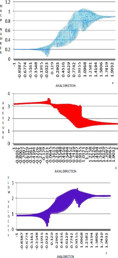
Fig. 1 The contours of Mach number, pressure and velocity in the passage at mid-plane (dimensionless), β1 = 90° 

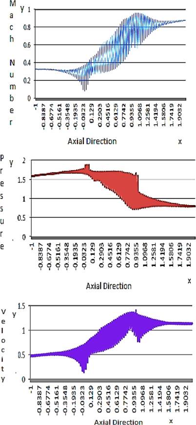
Fig. 2 The contours of Mach number, pressure and velocity in the passage at mid-plane (dimensionless), β1 = 120° 

The numerical and analytical Mach number distributions along the suction and pressure surfaces, plotted in Figs. 1 and 3, are in good agreement.

Fig. 3 Analytical Mach number distribution for stator blade cascade 

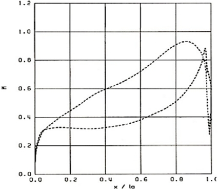
Fig. 4 represents the particle tracks released from the inlet domain, they show particle tracks and path lines for each base running.

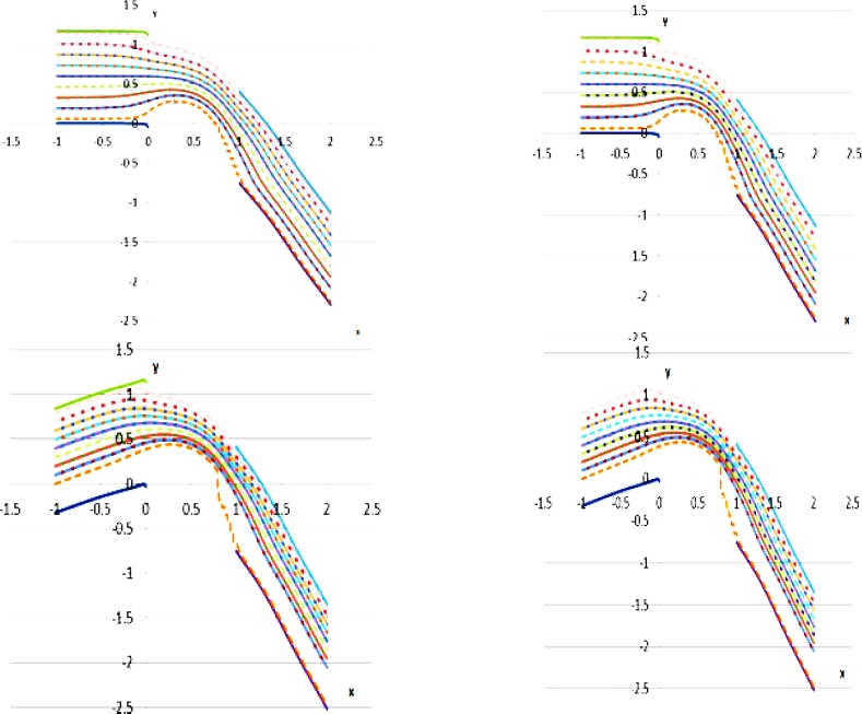
Fig. 4 Particle tracks and paths lines for base running (left), profile of velocity against position (right) 

Fig. 5 represents the velocity profiles of wet steam in the passage, the orange dot line reach the highest velocity value before the other dot lines. It represents the particle trajectory closer to the suction side and matches the orange dot line

Fig. 5 Velocity profiles of wet steam in the passage 

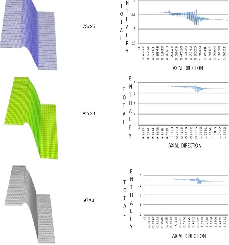
Fig. 6 illustrates the stability of computational calculation for wet steam flow in three sections of the channel. The flux increases in the zone of the throat where there is a change in geometrical and flow conditions then stability is almost achieved in the outlet plane.

Fig. 6 Wet steam flux on stator blade surfaces 

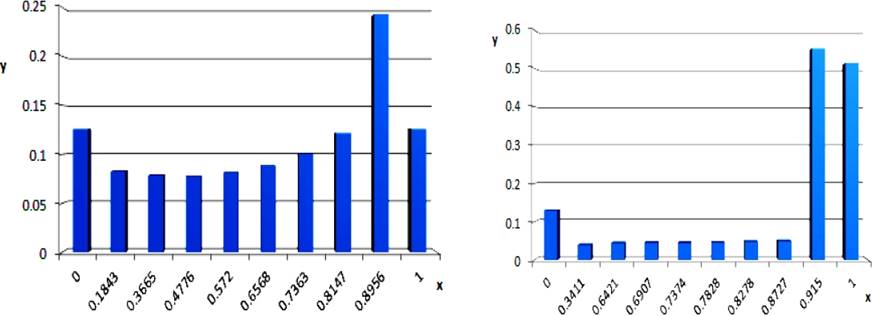
The areas in which moisture distributes along the pitch are shown in Fig. 7 and 8.

Fig. 6 Wet steam flux on stator blade surfaces 

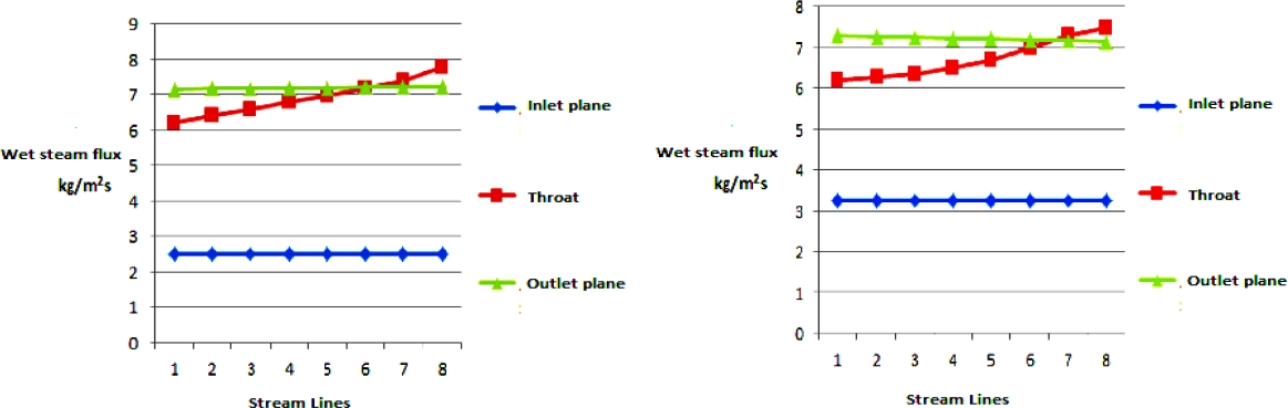
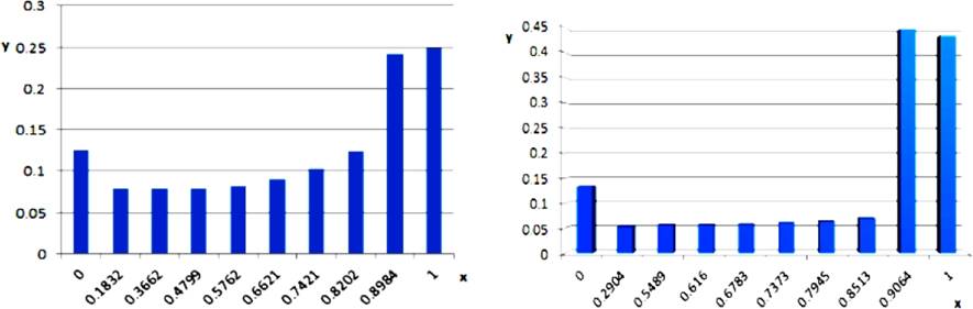
Fig. 7 Deposition as a function of pitch distance - x direction (dimensionless) in stator blades, dp = 0.25 µm, β1left = 90°, β1right = 120° 

Fig. 8 Numerical data of deposition as a function of pitch distance - x direction (dimensionless) in stator blades., dp = 1.0 µm, β1left = 90°, β1right = 120° 

5 Discussion

The FVM solver described is a mathematical and computational model that simulates the trajectories and velocities of water drops, as well as the distribution of mass of the particles. The numerical solution shows the maximum steam flow velocities reach 280 m/s (β1 = 90°) and 275.51 m/s (β1 = 120°) in the throat passage. The minimum value is in the leading edge, which corresponds to the stagnation point. The pressure distributions at the mid span are shown in Figs. 1 and 2. The maximum pressure on the leading edge has a value of 3.98 kPa (β1 = 90°) and 4.049 kPa (β1 = 120°), while the minimum is on the suction side in the throat region, see Table 2.

Table 2 Steam flow parameters 

Variations in steam flow angle and diameter of the particles were done to predict the quantity and distribution of the deposited water on stator blade surfaces. The concave surface of a blade can collect droplets by inertial impaction; shown in Figs. 7 and 8.

This effect was modeling taking the streamlines to be parabolic with a constant velocity component in the direction of the inlet flow as shown in Fig. 4. Ignoring the boundary layer, a numerical result was obtained for the collection of droplets in terms of direct inertia impaction.

The diameter changes from 0.25 µm up 1 µm. Most 0.25 µm particles move along with the steam flow consistently, and very few particles impact de inner arc of blade. When the inlet angles of flow are different, more 0.25 µm particles tend to impact the stator blade under the full load. By contrast, with the dominance of their inertia, 1 µm particles can be easily separated from steam flow and impact the stator blade surface at a high normal velocity [¹⁵].

As the diameter of the liquid particles increases, the deposition rate also increases reaching a maximum value near the trailing edge in the axial direction. The water deposition rises, changing from 6.0749 kg/m²s to 7.5 kg/m²s at the exit, this performance is caused by the fact that as diameter, flow angle and velocity increase, the amount of deposited particles increases.

Fig. 6 presents the curves of droplet deposition rate for the base running at each case. It is observed that maximum value is located at the trailing edge, see Table 3. This value reaches 7.92 kg/m²s and corresponds to the throat zone. In the leading edge the deposition rate is minimum compared with the throat zone, near to 2.5 kg/m²s.

Table 3 Deposition parameters 

By comparison, Q. Zhou, Na Li and co-workers [¹⁶] established a numerical framework that analyzed the movements of water drop in a blade channel based on the solution of the flow field of water steam in turbine, and statistics such as velocity and position were obtained as the working condition and particle size was varied. They developed a numerical tool to study the water drop erosion in turbine engines. Computational fluid dynamics and particle trace model in the Lagrangian Coordinates were employed to simulate the trajectories of water drop in a flow of wet steam in the blade channel.

6 Conclusions

The predictions reported in this paper contain the modeling of flow with changes of inlet parameters. The objective was to modify the existent flow a pattern, looking to understand the mechanism through which erosion and wetness loss develops and minimize their impact on blade surfaces. In the present work continuous-discrete phase model was used to predict the water deposition distribution on surface stator blades. Two-dimensional inviscid transonic flow was simulated using a cell-vertex finite volume space discretization method on structured triangular mesh. The steady state solution was reached by pseudo-time marching the Euler equations. Polynomial smoothing was used for convergence acceleration.

The effect of vapor mass flow rate, flow angle and diameter of the particle are studied by comparing the results, obtained by solving CFD problem.

The comparison shows that the effect of the variation of these parameters increases the deposition mechanism. The deposition distribution obtained varying flow angle and diameter of particles show that the values of surface deposition increase, while the drop diameter increases. The distribution of droplet deposition is fundamental information for solving and minimizing the wet steam effects in the steam turbines. Knowledge of the quantity and distribution of the deposited water is necessary if the operating life of the moving blades in a given turbine is to be predicted with any accuracy.