


 nova página do texto(beta)
 Inglês (pdf)
 Artigo em XML
 Referências do artigo
 Enviar este artigo por email
 Citado por SciELO
  Similares em
SciELO
Similares em
SciELO 
 Permalink
1 Introduction
Counting problems, although intrinsically interesting, have applications in a wide range of different areas. For instance, when estimating the probability that a given graph remains connected (graph connectivity is fundamental in network reliability theory) or when a propositional formula needs to be probabilistically tested to be true. The estimation of such probabilities can be seen as a counting problem. Counting problems also arise naturally in Artificial Intelligence Research, when some methods are used in reasoning areas, such as computing the ‘degree of belief’ when ‘Bayesian belief networks’ are used [6, 5, 17, 18].
Counting has become an important area in theoretical computer science, even though it has received less attention than decision problems. There is a handful of counting problems in graph theory that can be solved exactly in polynomial time, and indeed an important line of research is to determine low-exponential upper bounds for the time complexity of hard counting problems.
An edge cover of a graph G is a subset of edges covering all nodes of G. The problem of counting the number of edge cover sets of a graph, denoted as #Edge_Covers, is a #P complete problem proven via the reduction from #Twice-SAT to #Edge_Covers [4]. Most of the research on the subject has focused on approximate algorithms. In [2], an approximation algorithm for counting edge covers on 3 regular randomized graphs was presented.
More recently, in [13] a fully polynomial time approximation scheme (FPTAS) for counting edge covers of simple graphs was proposed; same authors have extended the technique to tackle the weighted edge cover problem in [14]. Additionally, the edge covering property was found interesting and relevant in various domains [7, 15, 16]. The edge cover polynomial of a graph G is presented in [1].
The edge cover problem is related to (perfect) matching, k-factor problems among others. The previous problems involve a set of edges satisfying local vertex constraints. For matching, it is at most one incident edge should be chosen compared to the edge cover problem in which at least one edge is chosen. For generic constraints, it is the Holant setting [10, 11], which has been studied for exact counting [9, 11, 8].
In this paper, we present an exact algorithm for counting edge covers taking into account that there exists a polynomial time algorithm for non-intersecting cyclic graphs [15]. Having said that, the technique is basically to reduce a simple graph into a sequence of non-intersecting cyclic graphs. The time complexity of the algorithm is also studied. Although, the complexity of our proposal remains exponential its complexity is smaller than the trivial 2(m−n), where m and n are the number of edges and vertices respectively of the input graph.
2 Preliminaries
A graph is a pair G = (V, E), where V is a set of vertices and E is a set of edges that associates pairs of vertices. The number of vertices and edges is denoted by v(G) and e(G), respectively. A simple graph is an unweighted, undirected graph containing no graph loops or multiple edges. Through the paper only simple finite graphs will be considered, where G is a finite graph if n = |v(G)| < ∞ and m = |e(G)| < ∞. A simple cycle in a simple graph is a set of vertices that can be arranged in a cyclic sequence in such a way that two vertices are adjacent if they are consecutive in the sequence, and are nonadjacent otherwise [3]. A cycle basis is a minimal set of simple cycles such that any cycle can be written as the sum of the cycles in the basis. A graph is said to be non-intersecting cyclic if any pair of simple cycles are edge disjoints.
An edge cover of a graph G is a set of edges C ⊆ EG, such that meets all vertices of G. That is for any v ∈ V, it holds that Ev ∩ C ≠ ∅ where Ev is the set of edges incident to v. The family of edge covers for the graph G will be denoted by 𝓔G. The problem of computing the cardinality of 𝓔G is well known to be ♯P-complete problem.
A subgraph of a graph G is a graph G′ = (V′, E′) such that V′ ⊆ V and E′ ⊆ E. If e ∊ E, e can simply be removed from graph G, yielding a subgraph denoted by G\e; this is obviously the graph (V, E − e). Analogously, if v ∈ V, G\v is the graph (V − v, E′) where E′ ⊆ E consists of the edges in E except those incident at v. A spanning subgraph is a subgraph computed by deleting a number of edges while keeping all its vertices covered, that is if S ⊂ E is a subset of E, then a spanning subgraph of G = (V, E) is a graph (V, S ⊆ E) such that for every v ∈ V it holds Ev ∩ S ≠ ∅.
A path in a graph is a linear sequence of adjacent vertices, whereas a cycle in a graph G is a simple graph whose vertices can be arranged in a cyclic sequence in such a way that two vertices are adjacent if they are consecutive in the sequence, and are nonadjacent otherwise [3]. The length of a path or a cycle is the number of its edges.
An acyclic graph is a graph that does not contain cycles. The connected acyclic graphs are called trees, and a connected graph is a graph that for any two pair of vertices there exists a path connecting them. The number of connected components of a graph G is denoted by c(G). It is not difficult to infer that in a tree there is a unique path connecting any two pair of vertices. Let T(v) be a tree T with root vertex v. The vertices in a tree with degree equal to one are called leaves.
2.1 The Cycle Space
A cycle basis is a minimal set of basic cycles such that any cycle can be written as the sum of the cycles in the basis [12]. The sum of cycles Ci is defined as the subgraph C1 ⊕ ⋯ ⊕ Ck, where the edges are those contained in an odd number of Ci’s, i ∈ {1, …, k} with k ∈ ℕ arbitrary. The aforementioned sum gives to the set of cycle or cycle space  the structure of a vector space under a given field k. The dimension of the cycle space 𝒞 is dimk 𝒞 = |𝓑| where 𝓑 is a basis for 𝒞. In particular, if G is a simple graph the field is taken to be k = 𝔽2, which is the case concerning this paper. Thus the field 𝔽2 will be used through the entire paper to describe cycle space of graphs.
3 Splitting Simple Graphs
The technique proposed in this paper, assumes that if the graph has cycles, it is always possible to calculate a cycle basis for the cycle space of the graph. The cycle basis to be considered in this paper can easily be constructed by using the well known depth first search algorithm (DFS) [3]. The process of getting a spanning tree for G by DFS algorithm will be denoted by ⟨G⟩. By using depth first search a spanning tree or forest T = ⟨G⟩ can be constructed for any graph G. The cycle basis is the set of all cycles such that each of them consists of an edge in  and the simple path in T connecting its two end vertices. The dimension of 𝒞G is therefore
  .
.
3.1 Non-intersecting Cycle Graph or Basic Graphs
In this paper we define basic graphs or non-intersecting cycle graphs as those simple graphs G with dim 𝒞G ≠ 0 in such a way that any pair of basic cycles are edge disjoints. Let 𝓑 = {C1, …, Ck} a basis for the cycle space 𝒞G; if Ck = (Vk, Ek) let us define the sequence of intersections of the edge sets {Ei} as
 (3.1)
(3.1)
for any Ip = {i1, …, ip} {1, …, k}, it is clear that 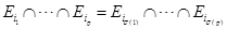 for any permutation σ ∈ Sp; where Sp is the symmetric group of permutations. The number of different terms to consider in Equation (3.1) is given by k!/(k − p)!p! which is the number of different combinations of the index set Ip. Thus, we can establish the conditions of whether a graph G has not an intersecting cycle basis. If the graph G is not acyclic and B2 = ∅ then dim G ≥ 1 so G is called a basic graph. Let e ∈ E be an edge and define ne as the maximum integer such that e belongs to as many as ne edge sets Ei. In other words, ne = max{p | Bp ≠ ∅}.
3.2 Splitting a Graph into Basic Graphs
Computing edge covers for simple graphs lies on the idea of splitting a given graph G into acyclic graphs or basic graphs. It will be shown, that calculating edge covers for simple graphs can be reduced to the computation of edge covers for acyclic graphs or basic graphs thus being able to fully compute |𝓔G|. The definition below describes in detail the process of splitting a graph into smaller graphs, which eventually leads to a decomposition of simple graphs into acyclic graphs or basic graphs.
Definition 1 For a given graph G = (V, E),
1. the split at vertex v ∈ V is defined as the graph G ⊣ v = (V′, E′) where
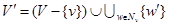 and
and 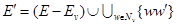 with w′ ∉ V,
2. the subdivision operation at edge e = uv ∈ E is defined as the graph G⊥e = (V ∪ {z}, (E − e) ∪ {uz, zv}) with z ∉ V, and z can be written either as uv or vu.
3. If e = uv ∈ E is an edge, G/e will denote the resulting graph after performing the following operation
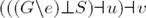
where S = Eu ∪ Ev − {e}. The subdivide operation (G\e) ⊥ S means tacitly (⋯((G\e) ⊥ f) ⊥ g ⋯)) where f, g, … ∈ S.
Above definition can be easily extended to subsets V′ = {v1, …, vr} ⊆ V, E′ = {e1, …, es} ⊂ E, that is G ⊣ V′ = (⋯((G ⊣ v1) ⊣ v2)⋯) ⊣ vr; analogously, G ⊥ E′ = (⋯((G ⊥ e1) ⊥ e2)⋯) ⊥ es. It must be noted, that the order on which the operations to obtain G/e are performed is unimportant as long as one keeps track of the labels used during the process.
Example 1 Consider the star graph W4 as presented in Figure 1.

If H, Q are graphs not necessarily edge or vertex disjoint we define a formal union of H and Q as the graph H ⊔ Q by properly relabelling VH and VQ; this can be accomplished by defining VH⊔Q = {(u, 1) | u ∈ H} ∪ {(u, 2) | u ∈ Q}. The edge set EH⊔Q could be defined as follows: if a, b ∈ VH⊔Q such that a = (u, i), b = (v, j) for some i, j ∈ {1, 2} and u, v ∈ VH ∪ VQ then ab ∈ EH⊔Q if and only if uv ∈ EH ∪ EQ and i = j.
Others labeling systems might work out just fine, as long as they respect the integrity of graphs H and Q. To recover the original graphs, we define the projections πX, as πH(H ⊔ Q) = H and πQ(H ⊔ Q) = Q; that is the projections πX revert the relabeling process to the original for both graphs H and Q.
Definition 2 Let G = (V, E) be a simple graph. Let us define the split operator ⊔e as
(i) the graph ⊔eG = G\e ⊔ G/e, that is the graph G splits into the graph G\e and the graph G/e if e ∈ E. If e ∉ E then ⊔eG = πG(G\e⊔G/e) = πG(G⊔G) = G.
(ii) if H, Q are arbitrary graphs then ⊔e(H⊔Q) = ⊔eH⊔ ⊔eQ with e ∈ EH ∪ EQ.
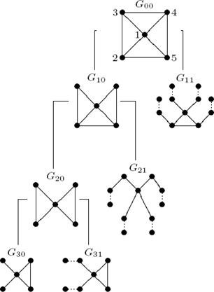
Example 2 Figure 2 shows an example of how a simple graph can be decomposed into acyclic or basic graphs.
3.3 Edge Covering Sets for Simple Graphs
The following results summarize the main properties of the split operator ⊔e, necessary for the calculation of the edge covering sets for simple graphs. The first result is regarding the dimension of the cycle spaces 𝒞G/e and 𝒞G for an edge e in the cotree of G. The proposition is rather simple in the sense that the resulting graph after applying G/e its dimension must diminishes certain amount which allow us to conclude that the operator ⊔ will split the graph G into non-intersecting cyclic graph.
Proposition 3.1 Let G be a simple graph,  a cycle base, e = uv ∈
  an edge in the cotree of G. If be = |𝓑u ∪ v| where u = {C ∈ 𝓑|u ∈ C} and 𝓑v = {C ∈ 𝓑|v ∈ C} then be + dim 𝒞G/e = dim G
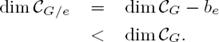
Proof 1 Every fundamental cycle containing either u or v must disappear under the operation G/e then those edges in that do not contain u or v are the only ones that contribute to the dimension of the graph G/e, therefore dim 𝒞G/e = dim 𝒞G − be.
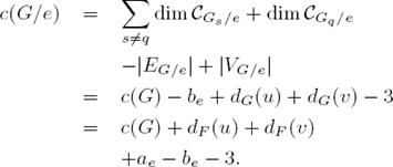
The proposition above allow us to explicitly calculate the number of connected components into which the graph G/e is being decomposed, on the other hand is providing a rather efficient way of testing whether or not G/e is a non-intersecting cyclic graph. The lemma below assumes that the graph in consideration is not connected, that is G has multiple connected components, thus we must consider a spanning forest for G instead of its spanning tree.
Lemma 1 Let G = (V, E) be a simple graph, F,  are a spanning forest and its corresponding coforest for G, respectively; let us choose an edge e = uv ∈ EG and consider the split ⊔eG of G. If ae = |(Eu ∪ Ev) ∩ | then
(i) If e ∈
then c(G\e) = c(G) and c(G/e) = c(G) + dF (u) + dF (v) + ae − be − 3.(ii) It holds that dim 𝒞G\e = dim 𝒞G − 1 and dim 𝒞G/e < dim 𝒞G.
(iii) There exists a bijective map ε : 𝓔⊔eG → 𝓔G. That is, if S is an edge covering set for G\e or G/e then ε(S) is an edge covering set for G, which is equivalent to 𝓔G = 𝓔G\e ∪ ε(𝓔G/e). Thus, |𝓔G| = |𝓔G\e| + |𝓔G/e|.
Proof 2 (i) For any forest F, |EF| = |VF| − c(F). If G = ⊕sGs, where Gs are the connected components of G, a spanning forest F for G is a disjoint union ⊕Ts such that Ts is an spanning tree for every component Gs. If e ∈ = ∪s s, where s = EGs − ETs, there exist q such that e ∈ q, e ∉ EGs and Gs\e = Gs with s ≠ q and therefore c(Gq\e) = c(Gq) which immediately implies that c(G\e) = c(G).
The operation G/e on G is clearly adding vertices and edges as follows: |VG/e| = |VG| + 2(dG(u) + dG(v)) − 6 for vertices and |EG/e| = |EG| + dG(u) + dG(v) − 3 for edges. It is not difficult to check that for any graph G, c(G) = dim 𝒞G − |EG| + |VG|, as a consequence we also have c(G/e) = dim 𝒞G/e − |EG/e| + |VG/e|. Since Tq is a spanning tree of Gq, by Proposition (3.1) dim 𝒞Gq/e = dim 𝒞Gq − be where 𝓑, the basis that defines be, is the basis for the cycle space 𝒞Gq; clearly we also have that dG(u) + dG(v) = dF(u) + dF(v) + ae then
(ii) By definition of the cycle space 𝒞Gs,
s forms a vector basis for every s, thus dim 𝒞Gs = || and since |ETs| = |VGs| − 1 we have that dim 𝒞Gs = |EGs| − |VGs| + 1. Now, if e ∈ then e ∈ q for some q; thus dim 𝒞Gq\e = |EGq\e| − |VGq\e| + 1, but |EGq\e| = |EGq| − 1 and |VGq\e| = |VGq| so we have that dim 𝒞Gq\e = dim 𝒞Gq − 1. On the other hand, since G = ⊕sGs we have that G\e = [Gq\e] ⊕ ⊕s≠q Gs and so a sum of cycle spaces 𝒞G\e = 𝒞Gq\e ⊕ ⊕s≠q 𝒞Gs such that

It readily follows from Proposition (3.1) that dim 𝒞Gq/e = dim 𝒞Gq − be where be as in Proposition (3.1) with 𝓑 replaced by 𝓑q, the fundamental basis for graph Gq. Now, be is always different form zero since 𝓑qu ≠ ∅ and 𝓑qv ≠ ∅ because they always contain the fundamental cycle formed by the edge e. Thus,
If e ∈ T for some T in the forest then there must exists C ∈ B such that e ∈ C. The cycle C is destroyed under the operation ⊔eG therefore dim 𝒞⊔eG < dim 𝒞G.
(iii) The family 𝓔G can be partitioned into two disjoint subfamilies of edge covering sets, that is 𝓡 = {S ∈ 𝓔G|e ∈ S} then 𝓔G = 𝓡 ∪ 𝓡c. To build up the map ε we proceed as follows: S ∈ 𝓡c if and only if S ∈ 𝓔G\e; this is because G\e ⊆ G thus any S ∈ 𝓡c must be a subset of EG\e and vice versa. Therefore, we define ε|𝓡c = id, where id is the identity map. Let Nz = {zi}i∈Iz be the set of adjacent vertices to z, Iz a set of indices of cardinality dG\e(z) where z is either u or v. Let us define Qz = {ziz′i} and Q′z = {z′iz″i}, thus any S ∈ 𝓔G/e must necessarily contain the set Q′z; if any f ∈ Q′z is not in S then S would not be an edge covering set because z″i will be an isolated vertex for some i ∈ Iz. So, S = Q′u ∪ Q′v ∪ S′ for some S′ ⊆ EG/e such that S′ ∩ Q′z = ∅ for z = u, v. Now if R ∈ 𝓡 then R = {e} ∪ R′ such that e ∉ R′. Since |EG/e| = |EG\e| + dG\e(u) + dG\e(v), and |EG/e − Q′u ∪ Q′v| = |EG/e| − |Q′u| − |Q′v| which implies that |EG/e − Q′u ∪ Q′v| = |EG\e| and therefore there exist a bijection φ between sets 𝒫(EG/e − Q′u ∪ Q′v) and 𝒫(EG\e) since they are both finite. In fact, φ can be chosen in such a way that if Q′u ∪ Q′v ∪ S′ ∈ 𝓔G/e then {e} ∪ φ(S′) ∈ 𝓡 and vice versa. Therefore, ε(Q′u ∪ Q′v ∪ S′) = {e} ∪ φ(S′) and ε−1({e} ∪ R′) = Q′u ∪ Q′v ∪ φ−1(R′).
The family 𝓔G\e accounts for those edge covering sets S for G on which e ∉ S whereas 𝓔G/e stands for those edge covering sets where e is always a member.
Let S ⊆ E be a subset of edges, from Definiton (2)(i) the split of G along S, denoted by ⊔SG, is recursively defined in terms of the sequence of splits Gij = ⊔eiG(i−1)j = G(i−1)j\ei ⊔ G(i−1)j/ei, i ∈ {1, ..., |S|} in particular for i = 1 we define G11 = G00\e1 ⊔ G00/e1 where G00 = G. By setting φ(i) = 2i−1 − 1 and for 0 ≤ j ≤ φ(i) we have therefore,
 (3.2)
(3.2)
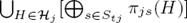
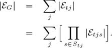
To short up the notation, we make G*tj = G(t−1)j * et, 𝓔tj = 𝓔Gtj and 𝓔*tj = 𝓔G(t−1)j*et = 𝓔G*tj with * ∈ {\, /}; under this notation we have that Gtj = G\tj ⊔ G/tj. In general, the graph Gtj is disconnected, if we denote by Gtjs its connected components then 𝓔tjs will denote the family of edge covering sets for each graph Gtj. For any given spanning tree T for a simple graph G, let us make t = || = dim 𝒞G, 𝓗j =  𝓔tjs for some set Stj ⊆ ℕ, where
  denotes the cartesian product and the projections will be denoted by πsj, for every s, j. Every edge covering set of a graph G induces a subgraph; if S ⊆ EQ by definition S meets all vertices of G then the induce graph of S becomes (VG, S). For the rest of the paper the family of edge covering sets, like 𝓔ijs will also denote the family of induced graphs by this sets. Therefore, the calculation of edge cover for a graph G is equivalent to calculate the induced graphs by edge covering sets, since most of the operations to be performed are graph operation like vertex splitting and edge subdivision.
Theorem 1 Let G be a finite, connected simple graph, T a spanning tree for G and denotes its cotree and t = || then
(i) the family {G\tj, G/tj}, appearing in the expansion ⊔
 G, are all acyclic graphs or non-intersecting cycle graphs for all j satisfying 0 ≤ j ≤ φ(t).
(ii) If G*tjs denotes the connected components of G*tj , then G*tjs are edge and vertex disjoint for every j, and G*tj =
 G*tjs for some set of indices Stj ∈ ℕ.
(iii) For every j, 0 ≤ j ≤ φ(t) there exist bijections εt :
 𝓔tj → 𝓔t, εtj : 𝓔tj → 𝓔(t−1)j such that 𝓔(t−1)j = 𝓔\(t−1)j ∪ εtj [𝓔/(t−1)j] and therefore
  .
.(iv) Let H = (H1, ..., H|St|j) ∈ 𝓗j be a vector of graphs of the cartesian product of family 𝓔tjs of induced graphs by edge covering sets, then 𝓔tj =
 and
and

For every q, 1 ≤ q ≤ t, there exist bijections εq
 (3.3)
(3.3)
in such a way that if ε = ε1 ◦ · · · ◦ εq then 𝓔G = ε(𝓔t) and
 (3.4)
(3.4)
Proof 3 (i) Let T be a spanning tree of G, = E\T its cotree and let I be an index set of integers. Let us consider ei ∈ , ui, vi ∈ VG such that ei = uivi; it is well known that ei and the path of T joining ui to vi forms a basic cycle. Let 𝓑 = {Ci}i∈I be that set of basic cycles then 𝓑 is a basis for the cycle space 𝒞G where Ci is the basic cycle corresponding to edge ei [12]. Let us define the family {Gtj} as in Equation (3.2) of Gt of subgraphs such that G00 = G, G*tj = G(t−1)j*et, j ∈ Ji and i ∈ I where Ji = {j|0 ≤ j ≤ φ(i), i ∈ I}. By making 𝒞*ij = 𝒞*Gij , it follows from Lemma (1), dim 𝒞\(i)(Ji) = dim 𝒞\(i−1)(Ji) − 1 and dim 𝒞/(i)(Ji) < dim 𝒞/(i−1)(Ji) for all i ∈ I. Therefore at some point in the decomposition process of graph G we must have dim 𝒞*tj = 0 or dim 𝒞*tj > 0 and B2(G*tj) ≠ ∅, which means that graphs G*tj are acyclic or non-intersecting cycle graphs for all j ∈ Jt.
(ii) It is clear from the definition of operator ⊔
that all graphs G*tj are vertex and edge disjoint. The connected components G*ijs are all subgraphs of G*tj thus G*ij = ⊕sG*ijs make sense.(iii) It follows from Lemma (1)(iii).
(iv) It follows from Lemma (1)(iii) and (i)-(iii) of this theorem.
Algorithm 1 decomposes the input graph into basic or acyclic graphs as Definition 1 establishes.

4 Time Complexity of the SPLIT Algorithm
Let G = (V, E) be a simple graph, m = |E|, n = |V|. The time complexity of Algorithm 1 is given by the recursive calls over G (steps 9 and 12) which can be established by the following theorem.
Theorem 2 Let G = (V, E) be a simple connected graph with m = |E|, n = |V| and nc = m − n + 1 the basic cycles of G. The recurrence which represent the complexity of Algorithm 1 is given by:
 (4.1)
(4.1)
whose solution is ≈ 1.46557
Proof 4 Since e is part of at least one pair of intersecting cycles, then G \ e = (V1, E1) is still a connected graph. |V1⊨n1=n, |E1| = m1 = m − 1. The number of base cycles in H1 is nc1 = m1 − n1 = m − n − 1 = nc − 1. Then, G \ e contains at least one pair less of intersecting cycles than G.
Let G/e = (V2, E2), n2 = |V2| and m2 = |E2|. By lemma 1-(i) nc−3. This recurrence has the characteristic polynomial p(r) = r3 − r2 − 1 which has the maximum real root r ≈ 1.46557.
Remark 1 Finding e such that e = uv ∈ E, e ∈ Bp(G) ≠ ∅ for some p has complexity O(m + n).
Corollary 1 The time complexity for splitting a simple graph G is given by:

A polynomial procedure for computing edge covers for basic graphs (acyclic or non-intersecting graphs) can be consulted at [15], so the complexity of counting edge covers is given by the splitting process.
5 Conclusions
A sound procedure has been presented to decompose a graph in order to compute the number of edge covers for the resulting subgraphs.
Regarding the cyclic graphs with intersecting cycles, a branch and bound procedure has been presented, it reduces the number of intersecting cycles until basic graphs are produced (subgraphs without intersecting cycles). Since polynomial time procedures are known for basic graphs, the computational complexity of the edge cover problem resides on intersecting cycle graphs.
Additionally, a recurrence relation has been deter-mined that establish an upper bound on the time to compute the number of edge covers on intersecting cycle graphs. It was also designed a “low-exponential” algorithm for the #Edge Covers problem whose upper bound is O(1.465571(m−n) * (m + n)), m and n being the number of edges and nodes of the input graph, respectively.

