1 Introduction

Path planning of agents (mobile devices including autonomous robots) consists in finding a sequence of motion tasks to reach a final goal in a known environment. Usually, constraints such as avoiding obstacles and collisions must also be satisfied. Constraints or specifications are usually given in a mathematical language, which traditionally has been a geometric one. It is then a natural research direction to study specification languages with more expressive power in order to give more complex instructions to agents.

Specifications involving sequentiality has recently been studied with great success in the setting of linear temporal logic [¹, ²³, ¹³, ¹⁴, ⁶, ²⁵]. Specification are written as linear temporal logic formulas, and plan generation corresponds to counterexample generation in a model checking tool: given a formula (specification) and a model (environment), find a path in the model not satisfying (the counterexample) the negation of a formula.

In the context of mobile robotics, it is often required to implement continuous trajectories. This is achieved by first giving a discrete abstraction of the robot environment, which can clearly be obtained by well known efficient decomposition methods for polygonal environments [²¹]. A discrete plan is then obtained from the discrete abstraction of the environment and the specification by means of model checking techniques. A continuous implementation of the discrete plan can be obtained with a hybrid control approach [¹¹].

As suggested by its name, linear temporal logic (LTL) formulas can express linear plans only. In linear plans, agents execute tasks in a linear sequential order. Consider for instance the following formula in linear temporal logic:

This expression requires a agent to visit p after one step, and after two steps to visit q. Hence, in a linear model, the above expression implies q is after p. However, in many cases it may not be true, say for instance that q is in a different path than p. Then, the resulting plan has a two branch tree form. With these kind of non-linear plans, more precisely branching plans, it is then easy to see that a team of agents may concurrently execute the plan, one agent each branch. In addition, since plans are tree shaped, collision-free plans are guaranteed and agents may be executed asynchronously.

In the community of context-aware computing, it has recently emerged the notion of context-aware path planning [²⁴], which concerns the path planning problem with particular context variables included in the set of constraints, as for instance, location, time, weather, and community sense.

For instance, for this last variable, a well-known scenario arises in the generation of evacuation plans. It is often the case that evacuation plans need to take in consideration a team of people (with an smart phone each or some). In this scenario, it is desirable, whenever possible, each (or at least some) people follow a different evacuation plan in order to avoid bottlenecks and expedite the evacuation. Branching tree planning in the evacuation scenario offers several distinct and collision-free evacuation plans.

In the current work, we study the µ-calculus, which is an expressive modal logic, in the context of branching path planning for mobile agents (devices, robots, etc.). The µ-calculus is one of the most expressive, yet computable, logic languages. The expressive power of the µ-calculus corresponds the bisimulation invariant fragment of monadic second order logic [⁵], and hence, by the Rabin’s Tree Theorem [²⁰], also corresponds to tree automata and regular languages (grammars).

The µ-calculus is also known as the queen of the program logics, because it subsumes the linear temporal logic LTL, the propositional dynamic logic PDL, the computational tree logic CTL, and many expressive descriptive logics [⁷].

2 A Modal Logic for Path Planning

In this Section, we present the propositional modal µ-calculus, which is an expressive modal logic equipped with least and greatest fixed-points. We also show how to use logic formulas as specifications for path planning. It is also formally defined the problem of path planning in terms of logic formulas and Kripke structures (graph models).

Through this paper, we consider countable sets only, hence, when written set, we denote countable set.

2.1 Syntax and Semantics

An alphabet or signature is a pair (P , X), such that

• — P is a set of propositional variables; and

• — X is a set of variables.

Unless otherwise stated, we consider a fixed alphabet.

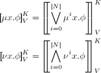
Definition 1 (Syntax). Given an alphabet, the set of µ-calculus formulas is given by the following grammar:

Formulas are interpreted as sets of nodes in Kripke structures (Definition 2). Intuitively, Kripke structures are graphs with labeled nodes, sometimes called transition systems. Propositions are true or false at each node, whereas negation and disjunction of formulas are interpreted as set complement and the union of sets, respectively. Modal formulas ⋄φ hold at nodes, such that there is at least one adjacent node where φ is true. µx.φ formulas are interpreted as least fixed-points. Intuitively, least fixed-points are used as operators for finite recursion.

Consider for instance formula ⋄p₃. In a graph model, this expression denotes nodes, such that there is at least one accessible node where p₃ is satisfied. Graphical representation of this example is depicted in Figure 1. ⋄p₃ holds in n₁ because n₃ is accessible from n₁ and p₃ is satisfied by n₃. Now consider the fixed-point formula µx.p₁ ∨ ⋄x. This formula is true at nodes where p₁ holds or at nodes that can access, through finite recursive navigation on edges, to at least one node where p₁ is true. In Figure 1, µx.p₁ ∨ ⋄x holds at nodes n₁, n₂, . . . , n_k. If we now consider formulas as specifications for mobile agents, then µx.p₁ ∨ ⋄x may be interpreted as a task for an agent, such that it must visit p₁ no matters how far p₁ is. Then the path traced by the formula can be seen as the path plan for the agent. However, it is natural to ask for another task, as for instance, also visit p₂ no matters how far it is, that is, µx.p₂ ∨ ⋄x. This two requirements may be easily expressed by conjunction:

Fig. 1 The interpretation of ⋄p₃, φ₁ = µx.p₁ ∨ ⋄x, and φ₂ = µx.p₂ ∨ ⋄x 

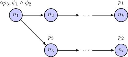
But it may also be the case that p₂ is not on the path to p₁, or the other way around (see Figure 1), that is, the plan is not linear. These two tasks may be performed by a team of two agents. In Figure 1, this conjunction of tasks holds at n₁ only, but µx.p₂ ∨ ⋄x is satisfied by n₁, n₃, . . . , n_l. This is the path to p₂ from n₁. Both paths, the one to p₁ and the one to p₂, form the non-linear plan required to do the tasks. Through this paper, we will show how to compute non-linear path plans. First, we give a formal description of formula semantics on Kripke structures.

Given an alphabet (P , X), a Kripke structure is a tuple (N, R, L), such that

• — N is a non-empty set of nodes;

• — R : N × N is a binary relations of nodes; and

• — L : N ↦ 2^P \ ∅ is a total label function.

A total Kripke structure is a Kripke structure where each node is connected by at least one transition relation, that is, for every node n ∈ N there is a relation R and a node n′ ∈ N, such that (n, n′) ∈ R. In this work, we consider total Kripke structures only.

Before giving an operational semantics of µ-calculus formulas, we need some notation. A valuation in a Kripke structure K is a function from the set of variables to the power set of nodes in K, that is, V : X ↦ 2^N. We write , when V(x) = S.

Definition 2 (Semantics). Given a Kripke structure K = (N, R, L) and a valuation V , formulas are interpreted as follows.

If , we say K satisfies φ. The model checking problem consists in automatically deciding whether or not a given Kripke structure satisfies a given formula. We say that a formula is satisfiable, if there is a Kripke structure satisfying the formula. In case there is no Kripke structure satisfying the formula, then it is said that the formula is unsatisfiable. When a formula is satisfied by any Kripke structure, the formula is valid.

Other traditional logic operators are defined as follows:

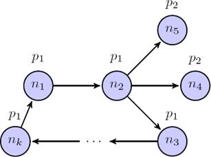
Conjunction is interpreted as expected, as set intersection. ⊥ is a contradiction. ◻φ holds at nodes where each adjacent node satisfies φ. Consider for instance formula ◻p₂, which denote nodes such that all its accessible nodes satisfies p₂.

In Figure 2, ◻p₂ does not hold at n₂, because although n₅ and n₄ are accessible nodes from n₂ and they satisfy p₂, there is one accessible node where p₂ is not satisfied and it is n₃.

Fig. 2 Infinite recursion: the interpretation of νx.p₁ ∧ ⋄x 

A greatest fixed point can also be defined as dual of the least fixed point.

This operator is intuitively used for non-finite recursion. Consider for instance formula νx.p₁ ∧ ⋄x. This formula denotes paths (finite or infinite) where p₁ is always true. In the context of path planning, it is natural to require a task to be performed permanently, such as surveillance. In Figure 2, νx.p₁ ∧ ⋄x denotes the cycle composed by n₁, n₂, n₃, . . . , n_k.

Due to Knaster and Tarski we know µ and ν formulas are fixed points. Before describing this well known result, we need some notation.

Definition 3 (Finite expansions). We define the finite expansion (approximants) of fixed-points as follows, for a natural number k.

We now recall the Knaster-Tarski Theorem in terms of finite expansions.

Theorem 1 (Knaster-Tarski Fixed-Point Theorem [²², ¹⁷]). For any Kripke structure K = (N, R, L) and a valuation V,

Other known operators in LTL and CTL can also be easily defined.

The until formula φ U ψ holds in each node of paths (adjacent nodes) where φ is true in all but he last node, where φ is satisfied. Release formula φ R ψ holds in nodes of paths where ψ is true in all but the last node, where φ is true. Also, release formula holds in each node of non-finite paths where ψ is always true.

2.2 Plans

Path plans for mobile agents are defined as the resulting trees of nodes satisfying a formula and its subformulas in a given Kripke structure. Consider for example the following formula:

This expression denotes a plan with two sub-tasks, the first one consists in, starting from p₀, visiting p₁ and p₂, in that order, whereas the second task also starts from p₀, but requires to visit p₃ and p₄, also in that order. In Figure 3, the Kripke structure satisfies the formula, the tree is the plan extracted from the Kripke structure that satisfies the formula together with its subformulas.

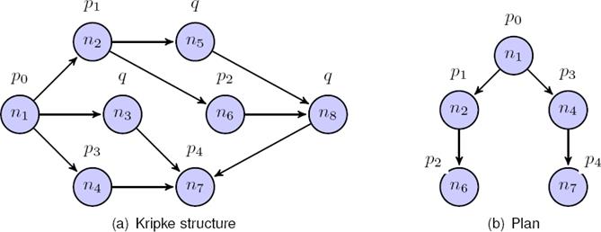
Fig. 3 A Kripke structure satisfying p₀ ∧ ⋄ (p₁ ∧ ⋄p₂) ∧ ⋄ (p₃ ∧ ⋄p₄), together with its corresponding plan 

As another example, consider now formula νx.p₁ ∧ ⋄x and its model displayed in Figure 2. The plan of the formula is then the one branched infinite tree composed by the infinite occurrence of paths composed by n₁, n₂, n₃, . . . , n_k.

That a satisfiable formula is satisfied by a tree shaped Kripke structure is a well known result.

Theorem 2 (Tree model property [⁷]). If a formula φ is satisfiable, that is, there is a Kripke structure K, such that for any valuation V we have that , then φ is satisfied by a tree shaped Kripke structure K′, that is, .

Before defining a path plan in terms of Kripke structures and formulas, we need some notation.

Definition 4. A tree on a Kripke structure K = (N, R, L), written T^K, is inductively defined as follows:

• — the empty tree ∅ is a tree; and

• — the tuple (n, T₁, T₂, . . . , T_k) is a tree, such that

• - n ∈ N is a node called the root,

• - for i = 1, . . . , k, T_i are trees, and

• - in case T_i is not empty, then R(n, n_i), where n_i is the roots of T_i, respectively.

When clear from context, we often simply write T for a tree.

We now define the notion of plan. Intuitively, a plan is a tree whose nodes satisfy, following the paths of the tree, a formula together with its subformulas.

Definition 5 (Plan). Given a Kripke structure K = (N, R, L) and a valuation V , we say a tree T^K on K is a plan for a formula φ if and only if T^K ⊨ φ, such that relation ⊨ is inductively defined as follows.

Relation ⊭ is defined as follows.

Because of the tree model property of µ-calculus (Theorem 2), we know that if there is model satisfying a formula, then there is also a plan (tree) satisfying the formula.

Corollary 1. If a formula φ is satisfiable, that is, there is a Kripke structure K, such that for any valuation V we have that , then there is a plan T^K for φ, that is, T^K ⊨ φ.

3 Path Planning

In this Section, we introduce a sequent-like system for the model checking problem, that is, given a formula and a Kripke structure, decide whether or not the Kripke structure satisfies the formula. Plans can be extracted from the proofs produced by the sequent system. It is also proven that the system is sound and complete.

The sequent system considered in this Section works with fixed-point alternation-free formulas in negation normal form. Occurrences of greatest and least fixed-points cannot then alternate. The negation normal form of a formula is defined as follows.

For the rest of the paper, when we refer to the negation of a formula ¬φ, we mean its negation normal form nnf(φ).

The set of subformulas of a formula is inductively defined as follows: if φ is a proposition, a variable or constant ⊤, then subformula(φ) = {φ}; if φ is a conjunction ψ ∧ ψ or a disjunction ψ ∨ ϕ, then subformula(φ) = {φ} ∪ subformula(ψ) ∪ subformula(ϕ); and if φ is a modal formula ⋄ψ or ◻ψ, or a negation ¬ψ, or a fixed point formula µx.ψ or νx.ψ, then subformula(φ) = {φ} ∪ subformula(ψ). The set of formulas in a modality is inductively defined as follows: mod(p) = mod(x) = mod(top) = {}; mod(⋄φ) = mod(◻φ) = subformulas(φ); mod(φ ∨ ψ) = mod(φ ∧ ψ) = mod(φ) ∪ mod(ψ); mod(¬φ) = mod(µx.φ) = mod(ν(.φ)) = mod(φ).

We say a formula φ occurs under the scope of a modality in another formula ψ, whenever φ ∈ mod(ψ). The set of free variables in a formula is inductively defined as follows: free(x) = {x}; free(⊤) = free(p) = {}; free(¬φ) = free(⋄φ) = free(◻φ) = free(φ); free(φ ∨ ψ) = free(φ ∧ ψ) = free(φ) ∪ free(ψ); and free(µx.φ) = free(νx.φ) = free(φ) \ {x}, provided x occurs in φ. We say a variable x occurs free in a formula φ, whenever x ∈ free(φ). Without loss of generality, we consider formulas where variables can only occur under the scope of a modality, and not free [⁵].

Sequents are defined as pairs, written n ⊢ ∆, where n is a node and ∆ is a (possibly empty) set of formulas. Intuitively, node n syntactically satisfies each formula in ∆. We say a sequent is empty if its set of formulas is empty.

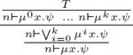
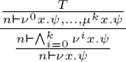
Rules are pairs (C, A), where C is a set of sequents, called consequent, and A is a family of sequent sets, called premises. Rules are usually written as follows:

Intuitively, from premises A, we derive C. If A contains only empty sequents, then we say A is empty and there are no premises. If a rule has no premises, then we say this rule is an axiom. A derivation system is composed by a set of rules.

Definition 6 (Planning derivation system). Given a Kripke structure K = (N, R, L), we define the following rules with respect to a given formula.

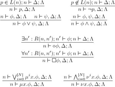
Please note that for readability we use commas for the union of formulas in sequents, and for the union of sequents we use semi-colons. That is, for a formula φ and a set of formulas ∆, we write φ, ∆ instead of {φ}∪∆, and for a sequent n ⊢ ∆ and a set of sequents Λ, we write n ⊢ ∆; Λ instead of {n ⊢ ∆} ∪ Λ.

Before defining derivation trees formally, consider the following formula evaluated in the Kripke structure displayed in Figure 3:

The corresponding derivation tree is the depicted in Figure 4. Inference goes bottom-up, so the formula in the bottom is concluded from the axiom (empty sequents). We thus read that n₀ ⊢ p₀ ∧ ⋄ (p₁ ∧ ⋄p₂) ∧ ⋄ (p₃ ∧ ⋄p₄) is concluded from n₀ ⊢ p₀, ⋄ (p₁ ∧ ⋄p₂) ∧ ⋄ (p₃ ∧ ⋄p₄) by applying the inference rule corresponding to conjunction of formulas. This last expression is concluded from n₀ ⊢ ⋄ (p₁ ∧ ⋄p₂) ∧ ⋄ (p₃ ∧ ⋄p₄) by applying the inference rule corresponding to propositions.

Fig. 4 A proof tree for p₀ ∧ ⋄ (p₁ ∧ ⋄p₂) ∧ ⋄ (p₃ ∧ ⋄p₄) in the Kripke structure of Figure 3  

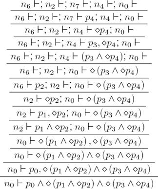
In this case, we know that p₀ ∈ L(n₀). It is now applied again the rule for conjunction, so for the premise we obtain n₀ ⊢ ⋄ (p₁ ∧ ⋄p₂) , ⋄ (p₃ ∧ ⋄p₄) Then, we apply the rule for diamond formulas, so the premise is n₂ ⊢p₁ ∧ ⋄p₂; n₀ ⊢ ⋄ (p₃ ∧ ⋄p₄). This is because we know that R(n₀, n₂).

Using conjunction rule, then the premise is now n₂ ⊢ p₁, ⋄p₂; n₀ ⊢ ⋄ (p₃ ∧ ⋄p₄), which is concluded from n₂ ⊢ ⋄p₂; n₀ ⊢ ⋄ (p₃ ∧ ⋄p₄) due to the proposition rule, in particular, because p₁ ∈ L(n₂).

Using again the diamond rule, the premise is then n₆ ⊢ p₂; n₂ ⊢; n₀ ⊢ ⋄ (p₃ ∧ ⋄p₄), because R(n₂, n₆). For the next step we obtain the axiom n₆ ⊢; n₂ ⊢; n₀ ⊢ ⋄ (p₃ ∧ ⋄p₄), because of proposition rule, more precisely, because p₂ ∈ L(n₆).

Analogously as just described above, we now apply successively the diamond, the conjunction and the diamond rule over n₀ ⊢ ⋄ (p₃ ∧ ⋄p₄) to finally obtain as premise n₆ ⊢; n₂ ⊢; n₇ ⊢; n₄ ⊢; n₀ ⊢, which turns to be an axiom.

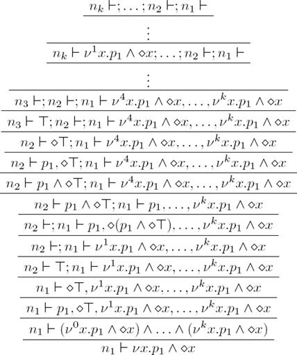
As another example, consider the corresponding proof tree in Figure 5 for νx.p₁ ∧ ⋄x in the Kripke structure in Figure 2.

Fig. 5 A proof tree for νx.p₁ ∧ ⋄x in the Kripke structure in Figure 2  

In order to formally define derivation trees, we will consider trees of sequents, that is, trees with sequents instead of nodes. Formally, given a sequent Λ and a derivation system, a derivation tree of Λ is a tree (Λ, T₁, T₂, . . . , T_k), such that

— T₁, . . . , T_k are all derivation trees of their respective sequent roots Λ₁, . . . , Λ_k, and

— is an instance of a rule in the derivation system.

We are now ready to formally define derivation trees satisfying a sequent for a given Kripke structure. Proof trees are derivation trees for a given sequent, such that a given Kripke structure satisfies the formula, intuitively, a proof tree containing finite branches with at least one ending with axioms.

Definition 7 (Proof tree). Consider the planning derivation system, a proof tree of a sequent Λ is a derivation tree of Λ, such that there is at least one branch ending with only empty sequents.

We are now ready to state the main result of this work, which is that the derivation system is sound and complete. This means that whenever there is a Kripke structure satisfying a formula, the derivation system obtains a proof tree.

Theorem 3 (Model Checking). A formula φ is satisfiable by a Kripke structure K, if and only if, there is a proof tree of n ⊢ φ, such that n is a node in K.

To prove the sequent system is correct, we need to show both directions of the double implication.

Theorem 4 (Completeness). If a formula φ is satisfiable by a Kripke structure K, then there is a node n in K, such that there is a proof tree of n ⊢ φ.

Proof. The proof goes by structural induction on the input formula.

First consider the input formula is a proposition p. We then know p ∈ L(n). Hence, n ⊢ p.

For the case of negation, recall formulas are negated normal form, hence, the scope of the negation symbol can only involve a proposition, say p. Since we know n satisfies ¬p, then p ∉ L(n), then n ⊢ p.

In case the input formula is a disjunction with form ψ ∨ ϕ, we know at least one of ψ or ϕ is satisfied by n. Without loss of generality, assume ψ is satisfied by n. Then by induction we know n ⊢ ψ, and hence n ⊢ ψ ∨ ϕ.

The case when the input formula is a conjunction is proven analogously as the case for disjunction.

Assume now the formula has the form ⋄ψ. Since n satisfies ⋄ψ, then there is at least one node n′ satisfying ψ, such that R(n, n′). By induction we obtain n′ ⊢ ψ and hence n ⊢ ⋄ψ.

The for modal formulas is proven analogously as the case of diamond formulas ⋄ψ.

We consider now the case when a least fixed-point µx.ψ is satisfied by n. By the Knaster-Tarski Fixed-Point Theorem 1, we know µx.ψ is equivalent to its finite expansion µⁱx.ψ where k is the number of nodes in K (Definition 3). We then obtain n satisfies the finite expansion. Hence, there is some i, such that n satisfies µⁱx.ψ. A second induction on the structure of µⁱx.ψ is applied in order to obtain n ⊢ µⁱx.ψ. These cases are identical as the ones already proven above. We then obtain n ⊢ µⁱx.ψ, hence n ⊢ µx.ψ.

Finally, for the case of greatest fixed points we proceed analogously as for least fixed points. By the Knaster-Tarski Fixed-Point Theorem 1, we know νx.ψ is equivalent to its finite expansion νⁱx.ψ, where k is the number of nodes in K (Definition 3). In order to show there is a proof tree of the finite expansion we proceed by induction on i (the number of conjuncts). For each step of the induction on i, we also apply another induction on the structure of ψ. By assumption, we know n satisfies ν⁰x.ψ, the base cases (when ψ is a proposition or a negated proposition) are trivial. Consider now ψ is of the form ⟨m⟩ ϕ, then there is a m-connected node n′ to n satisfying ψ, by induction we obtain n′ ⊢ ψ. n ⊢ ⟨m⟩ ψ follows immediately. Since variables only occur under the scope of a modality and not free, and the fixed-points cannot alternate, other cases go smoothly by structural induction. We now consider the inductive step on i. In order to show n ⊢ νⁱx.ψ, we again proceed by structural induction on ψ. Base cases are immediate. If ψ is ⟨m⟩ ϕ, it is not hard to see there is a m-connected node n′ to n, such that n′ ⊢ ϕ , which clearly implies n ⊢ ⟨m⟩ ϕ . n′ ⊢ ϕ is obtained by induction on ϕ. In the base case, n′ ⊢ follows from n′ ⊢ νⁱ⁻¹x.ϕ, which is known by induction. Other inductive cases goes straightforward by considering all possible occurrences of x. We then conclude n ⊢ νⁱx.ψ.

We now show the converse, that is, if we have a proof tree, then the formula is satisfiable by the Kripke structure.

Theorem 5 (Soundness). Given a Kripke structure K and a formula φ, if there is a proof tree of n ⊢ φ for some node n in K, then n ∈ for any valuation V.

Proof. We proceed in this proof also by structural induction on the input formula.

If the formula is a proposition p, we then know p ∈ L(n), then n satisfies p.

When the formula is a negation, then it has the form ¬p (recall formulas are in negated normal form). We then know p ∉ L(n), and then n does not satisfy p, hence n satisfies ¬p.

Consider the case of n ⊢ ψ ∨ ϕ. The proof tree has then the following form:

By induction we know that n ∈ or n ∈ for any V , then n ∈ .

Conjunction is proven analogously as disjunction.

If the input formula is ◻ψ, then the proof has the form

for all n₁, . . . , n_k ∈ N, such that R(n, n_i). Then by induction, n_i=1,...,k ∈ for any V , and hence n ∈ .

When the input is a diamond formula we proceed analogously as with box formulas.

Now, consider the case of µx.ψ. The proof has the following form:

for natural number k, which is the cardinality of set of nodes in K. We know there is some i, such that n ⊢ µⁱx.ψ. However, we cannot use direct induction to show that n ∈ for any valuation V, because µⁱx.φ is not a subformula of µx.φ. We then proceed to use a second induction, now on the structure of µ^kx.φ. These cases are proven as the ones already proven above. Finally, we obtain n ∈ .

The case for greatest fixed-points is proven in an analogous manner as the case for least fixed points. We know by assumption

for natural number k, which is the cardinality of set of nodes in K. We proceed by a second induction, now on the structure of νⁱx.φ, in order to show n ∈ for all i. These cases are proven as the ones already proven above (recall fixed points cannot alternate). We then conclude n ∈ .

Since nodes are syntactically represented in proof trees, and node transitions are denoted by derivation rules corresponding to modal formulas (diamond and box), it is not hard to see that plans can be extracted from proof trees. Consider for instance the proof tree in Figure 4. The nodes involved in the plan are n₀, n₂, n₆, n₄ and n₇. Transitions are denoted by the application of rules involving modal subformulas, hence we obtain that R(n₀, n₂), and R(n₂, n₆), in that order, and R(n₀, n₄) and R(n₄, n₇).

It is then easy to see that the plan is a two-branch tree composed by n₀, n₂, and n₆, and n₀, n₄, and n₇. A graphical representation of the branching plan over the proof tree of Figure 4 is depicted in Figure 6, where the bold transitions (diamond rules) defines the topology of the branching plan. In case there are not finite branches to extract a plan, we then extract the plan from the branch producing a ν-cycle. For instance, in Figure 5, from the branch producing the cycle is easy to extract the plan, which involves n₁, n₂, . . . , n_k, in that order.

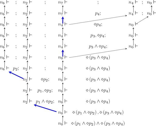
Fig. 6 A logical flow graph for ⋄ (p₁ ∧ ⋄p₂) ∧ ⋄ (p₃ ∧ ⋄p₄): Kripke structure of Figure 3, proof tree of Figure 4  

In order to formalize the plan extraction process from proof trees, inspired from the notion of logical flow graphs [⁹], we now define a similar notion for nodes occurring in proof trees. From this logical graphs, we are then going to be able to directly obtain plans in the name of tree paths.

Definition 8 (Logical graphs). Given a proof tree of a certain formula, we define a logical graph as a tuple (N, E), such that

The logical graph of the proof tree displayed in Figure 3 is shown in Figure 6.

A tree path is simply the resulting tree of a logical graph without considering repetitions.

Definition 9 (Tree path). Given a logical graph (N, E) of a proof tree of a formula φ, such that n ⊢ φ is the root of the proof tree, we inductively define a tree path φ starting from n as follows:

The tree path corresponding to the logical graph of proof tree in Figure 3 is graphically represented by the bold transitions in Figure 6.

Now, it is easy to imply from Theorem 3 that tree paths (Definition 9) are also plans (Definition 5).

Theorem 6 (Path planning). If there is a proof tree of a formula φ, then a tree path of φ is also a plan.

Proof. The proof goes by induction on the structure of the input formula φ.

If the input formula is a proposition p, then we know there is a node n, such that n ⊢ p. Hence, p ∈ L(n), and then n ⊨ p.

Negation, since it only occurs in front of propositions, is proven analogously as the case of propositions.

Consider now the input formula is a disjunction ψ ∨ ϕ. We then know that there is a proof tree for either n ⊢ ψ or n ⊢ ϕ. Without loss of generality assume there is a proof tree for n ⊢ ψ. By induction we then obtain there is plan (n, T₁, . . . , T_k) for ψ, that is, (n, T₁, . . . , T_k) ⊨ ψ. By definition of plan (Definition 5), then (n, T₁, . . . , T_k) ⊨ ψ ∨ ϕ.

The proof for the case of conjunctions is analogous as the proof for the case of disjunctions.

If the formula in question is ⋄ψ, and we know n ⊢ ⋄ψ, then there is a node n′ ⊢ ψ, such that R(n, n′). By induction, it is known there is a plan T′ = (n′, T₁, . . . , T_k) ⊨ ψ. Then, by Definition 5, we obtain a plan (n, T′) ⊨ ⋄ψ.

Due to the well known equivalence (Theorem 1, for the case of least fixed points µx.ψ, we prove for the corresponding finite expansion µⁱx.ψ, where k is the number of nodes of the Kripke structure satisfying the input formula. By assumption we know there is some i, such that n ⊢ µⁱx.ψ. A plan (n, T₁, . . . , T_m) ⊨ µⁱx.ψ is obtained by applying a second structural induction on µⁱx.ψ. This proof is the same as the cases already proven above. Now, by Definition 5, we obtain (n, T₁, . . . , T_m) ⊨ µⁱx.ψ.

Similarly as it is proven the least fixed point case, it is for the greatest fixed point.

4 Conclusions

Branching path planning for mobile agents are studied in the setting of the modal µ-calculus. In contrast with linear plans, where tasks are performed in a linear sequential order, in branching plans, several linear plans can be performed concurrently and asynchronously by a team of agents. Since plans are tree shaped, it is then guaranteed agents never collide. Since the µ-calculus is one of the most expressive, yet computable, formalisms, complex specifications for agents can be denoted by logic formulas. In particular, specifications involving finite and infinite recursion are nicely capture by the least and greatest fixed-points of the µ-calculus. In contrast with traditional plan generation in the context of temporal logics, where plans are obtained from counterexample generation in model checking tools, in the current work, we develop a model checking algorithm based on a sequent derivation system. This system produces proof trees whenever a formula is satisfied by the model. Plans are then directly extracted from the proof trees with the use of logical flow graphs. We provide correctness proofs for both, model checking and plan generation.

The inference system proposed in the current work is a general approach for non-linear plan generation. It can then be applied in motion planning for mobile robots by means of well-known discrete abstraction of the continuous environments typically occurring in robotics applications. We are also interested in the study of the application of our proposal in the setting of context-aware navigation systems for mobile devices.

Other further immediate research perspectives concerns the study and development of implementation techniques for the sequent system provided in this paper. In particular, we are interested in the representation of models based in binary decision diagrams [¹⁹]. We also expect to extend the approach proposed in the current paper, for the case of more expressive logics involving arithmetical constraints [⁴, ³, ²].