1 Introduction

The model used to represent digital binary volumes (or 3D binary images) is one of the most important research topic in computer graphics, looking for a better compression for storage, analysis or visu-alization purposes. Moreover, there are several demanding neighborhood operations on binary volumes such as connected-component-labeling (CCL), connectivity, collision detection, between others, where the performance variability of the existing algorithms is mainly caused by the number of basic geometric elements to analyze (voxels, triangles, planes, vertices, etc.).

In most of the reported literature, the operations to study binary volumes are performed directly on the classical voxel model [³¹, ⁴¹]. However, in the field of volume analysis and visualization, several alternative models have been devised for specific purposes. For instance, Hierarchical structures such as octrees and kd-trees have been used for Boolean operations [⁴⁶], CCL [¹⁷], and thinning [⁴⁰, ⁵⁸]. Octrees are used as a means of compacting regions and getting rid of the large amount of empty space in the extraction of isosurfaces [⁵⁷]. Kd-trees have been used to extract two-manifold isosurfaces [²⁴].

There are other models that store surface voxels, thereby gaining storage and computational efficiency. The semi-boundary representation affords direct access to surface voxels and performs fast visualization and manipulation operations [²⁵]. Certain methods of erosion, dilation and CCL use this representation [²⁰, ⁵¹].

On the other hand, a binary voxel model represents an object as the union of its fore-ground voxels and its continuous analog is an orthogonal pseudo-polyhedra (OPP) [³³]. OPP have been used in 2D to represent the extracted polygons from numerical control data [³⁹]. Some 3D applications of OPP are: general computer graphics applications such as geometric transformations and Boolean operations [¹⁰, ¹⁹], skeleton computation (instead of iterative peeling techniques) [¹⁸, ³⁷], and orthogonal hull computation [⁸, ⁹]. OPP have been also used in theory of hybrid systems to model the solutions of reachable states [¹⁰, ¹⁶].

The Extreme Vertices Model (EVM) and the Ordered Union of Disjoint Boxes (OUDB) [¹, ³] represent OPP in a compact way. EVM stores only a sorted subset of vertices of the OPP boundary, whereas OUDB keeps a sorted list of boxes that compose the whole object. EVM has been used to prove the suitability of OPP as geometric bounds in CSG [², ¹], and for many other 3D applications such as: erosion and dilation operations [⁴²], skeleton computation [⁴], virtual porosimetry without skeleton computation [⁴⁴], biomaterials structural parameters computation [⁵⁴] and model simplification [¹⁵]. OUDB has been used to perform CCL [⁵, ⁴²] and also for biomaterials structural parameters computation such as connectivity [⁷] and center of gravity [⁶].

In this paper we present in detail the Compact Union of Disjoint Boxes (CUDB), a representation model for OPP, and thus for binary volumes, that has been recently introduced, but without going into details of its implementation [¹⁴, ⁴⁴]. CUDB is a special kind of cell decomposition representation which performs a spatial partition of the volume in a non-hierarchical sweep-based way consisting of a set of disjoint boxes. This model is an improved version the OUDB. We test and report the performance of CUDB and also present new algorithms for CCL and collision detection.

The paper is arranged as follows. The next section reviews related work. Section 3 introduces CUDB using the object-oriented paradigm presenting algorithms for conversion to and from other models, and for basic computations as area and volume. Section 4 presents a new CUDB-based algorithm for CCL based on the detection of connected components in graph theory. Section 5 presents a collision detection algorithm for scenarios with multiple CUDB-represented objects. Sections 6 shows the performance of all the proposed algorithms by discussing experimental results. Finally, Section 7 concludes the paper and outlines future work.

2 Background and Related Work

The classical voxel model is based on a regular decomposition of the 3D space into a set of identical cubic cells called voxels. In a voxel model, voxels are all the same size and their edges are parallel to the main axes. Formally, a voxel model V of size n_x × n_y × n_z is defined as:

where v_i,j,k is a voxel in location (i, j, k).

From V , all geometric and topological information can be obtained. On each voxel v_i,j,k, there is a set of associated values. For a binary voxel model, the associated value of its voxels is limited to v_i,j,k ∈ {0, 1}, where 0 corresponds to the background and 1 to the foreground.

Algorithms for the voxel model are straightfor-ward to implement. However, just because of the size of the source models, it has the drawbacks of the loss of geometric information and high memory and computational power requirements [³²]. To reduce the memory footprint and the computation time of the algorithms, many alternative models have been proposed such as hierarchical data structures and boundary representations.

Hierarchical structures made recursive subdi-visions of the volume. In bintrees [⁴⁷] an axis-aligned hyperplane intersects the interior of the volume producing two equal parts. The Binary Space Partition (BSP) trees [⁵⁰] are similar to bintrees except that the position and direction of the subdivision hyperplanes are usually selected following an optimization heuristic. Octrees [¹¹], like bintrees, begin with an initial volume, but it create eight sub-volumes of equal size. And kd-trees [²⁴] are a special case of bintree, where each level is asymmetrically divided in alternate directions according to a discriminant (e.g., X, Y or Z-coordinate). In this structures, volume subdivision is repeated until a certain satisfactory level of refinement or until achieving the maximum level of recursion.

When working with binary volume datasets, it is not necessary to keep the exact scanned density values. Therefore, boundary models are also adequate to represent these kind of datasets. The basic model for representing the polygonal surface of an object is the Boundary Representation (B-Rep) model [³⁸] that keeps explicitly all of the relationships between geometric elements such as vertices, edges and faces. However, there are many proposed models for representing the object boundary in a more compact way.

Semi-boundary (SB) [⁵²] is a data structure which stores only the boundary voxels of the volume keeping the information of the interior voxels in an implicit way. Shell representation [⁵³] has the same indexing scheme used in the SB representation, but the set of voxels, which belongs to the list that contains all the boundary voxels of the volume, was redefined in order to represent objects with fuzzy boundaries. Cell-boundary [³⁴] is also a very similar representation to SB, which consists of a set of boundary cells with their voxel configurations, so, the points of the sample in SB become vertices of the cells in the cell-boundary representation.

2.1 EVM and OUDB models

The Extreme Vertices Model (EVM) [², ³] is a very concise representation scheme in which any OPP can be described using a subset of its vertices: the extreme vertices. EVM is actually a complete solid model with very fast Boolean operations, it is an implicit B-Rep model, i.e., all the geometry and topological relations concerning faces, edges and vertices of the represented OPP can be obtained from the EVM [⁴³] and therefore represents OPP unambiguously [⁵⁵].

Let Q be a finite set of points in ℝ³, the ABC-sorted set of Q is the set resulting from sorting Q according to A-coordinate, then to B-coordinate, and then to C-coordinate. Let P be an OPP, a brink is the maximal uninterrupted segment built out of a sequence of collinear and contiguous two-manifold edges of P and its ending vertices are called extreme vertices (EV). An OPP can be represented in a concise way with the ABC-sorted set of its EV and such representation scheme is called EV.

The Ordered Union of Disjoint Boxes (OUDB) [¹, ⁴²] is a special kind of spatial partitioning representation derived from EVM, where an OPP is decomposed in a list of disjoint boxes. EVM can be obtained from the voxel model, in turn, OUDB is obtained from EVM. The conversions algorithms have been published [⁴²]. To introduce later the CUDB model, we first briefly introduce OUDB.

Let P be an OPP and Π_c a plane whose normal is parallel, without loss of generality, to the X axis, intersecting it at x = c, where c ranges from −∞ to +∞. Then, this plane sweeps the whole space as c varies within its range, intersecting P at certain intervals. Let us assume that this intersection changes at c = C₁, ..., C_n. More formally, , ∀i = 1, ..., n, where δ is an arbitrarily small quantity. Then, is called a cut of P and , for any C_s such that C_i < C_s < C_i+1, is called a section of P .

Fig. 1 shows an OP with its cuts and sections perpendicular to the X axis. Since we work with bounded regions, S₀(P) = ∅ and S_n(P) = ∅, where n is the total number of cuts along a given coordinate axis.

Fig. 1 (a) An orthogonal polyhedron with 5 cuts. (b) Its sequence of 4 prisms with the representative sections (X direction) 

Cuts and sections are orthogonal polygons embedded in the 3D space. For each main direction, sections can be computed from cuts and cuts from sections by applying simple XOR operations. These operations are actually performed on the projections of cuts and sections onto the main plane parallel to them. From now on, we thus call the projection of the ith cut and ith section onto the main plane parallel to them C_i and S_i respectively.

The two following expressions relate cuts and sections:

(1)

(2)

where ⊗ denotes the regularized XOR operation. An OP can be represented with a sequence of orthogonal prisms represented by their section (see Fig. 1(b)). Moreover, if we apply the same reasoning to the representative section of each prism, an OP can be represented as a sequence of boxes.

The OUDB model represents an OPP with such a sequence of boxes. OUDB is axis-aligned like octrees and bintrees, but the partition is done along the object geometry as in BSP. Depending on the order of the axes along which we choose to split the data, an OPP P can be decomposed into six different ABC-OUDB, i.e., P is subdivided by planes perpendicular to the A-axis first, and then by planes perpendicular to the B-axis. Their corresponding sets of disjoint boxes are generally different. Fig. 2 shows the possible OUDB decompositions for the OPP in Fig. 1(a).

Fig. 2 The six possible OUDB decompositions for the OPP in Figure 1(a)  

3 Compact Union of Disjoint Boxes

Like OUDB, CUDB is also a union of disjoint boxes but a more compact one as several contiguous boxes are merged into one in several parts of the model. Let P be an OPP, to obtain the ABC-OUDB model, P is subdivided by planes perpendicular to the A-axis first, and then by planes perpendicular to the B-axis, at each cut C_i of P . Thus, every C_i splits all the geometry of P along the corresponding plane, and therefore some local regions of P , with which C_i actually has no relationship, are further unnecessarily divided. Fig. 3 shows this situation for the YZX-OUDB of an OPP P , where some cuts force unnecessary divisions. For OUDB this constraint is mandatory to keep sorted the resulting boxes. However, in order to subdivide just the pieces of P related with the cut which induces the splitting, this constraint can be relaxed.

Fig. 3 (a) An OPP. (b) YZX-OUDB with 16 boxes labeled according to their YZX-coordinates 

Formally, let P be an OPP. The CUDB(P) can be obtained by merging boxes in several parts of the corresponding OUDB(P). Then, this model is the set of boxes obtained according to the next properties:

The first property merges all unnecessary subdi-visions along B-axis. Following with the previous example, Fig. 4(a) shows that the pairs of boxes (2, 4), (7, 8), (9, 12), (11, 13) and (15, 16) depicted in Fig. 3(b) can be merged applying this property for the Z-axis.

Fig. 4 (a) Result after first merging in Z-direction. (b) Resulting YZX-CUDB with 7 boxes after merging in Y-direction 

The second property merges the remaining unnecessary subdivisions along A-axis. Following with the same example, the resulting model depicted in Fig. 4(b) shows that applying this second property for the Y-axis, not only the pairs of boxes (5, 8), but also the set of boxes (2, 6, 9, 10) depicted in Fig. 4(a) can be merged.

Then, the CUDB-representation of an OPP P , is the set of disjoint boxes of the corresponding OUDB, conveniently reduced by applying the two previous merging properties. Let β_i be a box in CUDB(P):

(3)

where n_b is the number of boxes, which is less or equal than the number of boxes in OUDB(P).

Like OUDB, there are six different ABC-CUDB models for a given OPP and the number of obtained boxes depends on the order of the axes along which we choose to split the data, but we cannot know it a priori. Boxes in CUDB are sorted according to its coordinate A, then to coordinate B, and finally to coordinate C of its lower bound.

Although the implicit order among boxes in OUDB that defines their adjacency is lost, preserving the adjacency information in the CUDB model is easy with a tiny storage effort. Each box has neighboring boxes in only two orthogonal directions: A and B-direction, and for each one there are two opposite senses, so, four arrays of pointers to the neighboring boxes (two for each direction) are enough to preserve the adjacency information that is required for future operations. We define these arrays as A-backward neighbors (ABN), A-forward neighbors (AFN), B-backward neighbors (BBN) and B-forward neighbors (BFN).

CUDB has been implemented as an object with a set of properties and methods. Next, we describe the CUDB object and the algorithms for conversion to and from EVM.

3.2 CUDB Computation

In order to obtain the CUDB-representation it is not necessary to have or compute the OUDB model. CUDB can be computed directly from the EVM, and the merging of boxes is performed on the fly. The strategy is similar to the process to compute OUDB [⁴²]. Cuts of the EVM-represented OPP are obtained sequentially, and sections are computed from them. When this process is performed in 2D, the corresponding sections result in the boxes of the OUDB model.

For the EVM to CUDB conversion method, the same set of boxes is computed on the fly and a box is stored in the CUDB model if it is not possible to merge it with previously computed boxes applying the aforementioned Properties 1 and 2.

For a given box, the set of previous boxes that have to be considered for merging with it are those boxes belonging to the previous A-slice, which can be adjacent in A-direction, and those boxes belonging to the previous B-slice, which can be adjacent in B-direction. To facilitate this process, temporary arrays of box pointers of the current and previous slices are maintained. The corresponding algorithm is detailed next.

As most of the algorithms dealing with EVM, the corresponding conversion algorithm is also recursive over the dimension. The main function EVMtoCUDB() (Algorithm 1) receives an EVM-represented OPP P and a flag to indicate if the adjacency relationship among boxes allows non-manifold configurations, and returns the CUDB-represented OPP Q containing the neighborhood information. This function initializes the temporary arrays of box pointers prevBBoxes, currentBBoxes, prevABoxes and currentABoxes, which are defined as global variables throughout the whole conversion process, and starts the recursion by calling the function doConversion() (Algorithm 2) with the original EVM-represented object P .

In function doConversion(), when dimension is 3D, the object is split at each cut in A-direction obtaining a set of 3D A-slices, , where n is the number of A-slices. Then the algorithm applies recursively to the 2D section representing each slice, which is split at every internal cut in B-direction obtaining a set of 2D B-slices, , where m is the number of B-slices represented by their 1D sections, which are composed by a set of collinear brinks in C-direction. Each of these brinks defines a box. Then, each 2D slice defines one o more boxes, and each 3D slice contains all the boxes defined in its 2D slices.

In the base case, when dimension is 1D, each brink in the current slice results in a box, which is inserted into currentBboxes. Boxes in a 2D slice can be merged with boxes in the previous slice , then, in the backtracking step of the recursion when dimension is 2D, function mergeB() (Algorithm 3) is called, which compares all boxes β₁ in currentBboxes with all boxes β₂ in (stored in prevBBoxes) for merging. In this process, when merging property 1 is accomplished, β₂ = β₂ ∪ β₁, and it is inserted into a array called activeBoxes. Otherwise, β₁ is inserted into currentABoxes and activeBoxes. When the process finishes, the array activeBoxes becomes prevBBoxes in order to be compared with boxes in in the next call.

Similar to the merging case in B-direction, boxes in a 3D slice can be merged with boxes in the previous slice . Once all the boxes of the current slice have been computed and conveniently merged in B-direction, they are in currentAboxes. Then, in the backtracking step of the recursion when dimension is 3D, function mergeA() (Algorithm 4) is called, which compares all boxes β₁ in currentAboxes with all boxes β₂ in (stored in prevAboxes) for merging. The steps in this function are quite similar to those in function mergeB(), but in this case, the merged boxes are finally inserted into the CUDB model Q.

Note that, the adjacency information of boxes (ABN, AF N, BBN, BF N) is computed on the fly when tests for merging are performed.

3.3 CUDB to EVM Conversion

As in OUDB, all of the boxes in CUDB are disjoint, and according to the following EVM property:

• — Let P and Q be two OPP such that P ∩^∗ Q = ∅, having EVM(P) and EVM(Q) as their respective models, then EVM(P ∪^∗ Q) = EVM(P) ⊗^∗ EVM(Q).

Therefore, a simple XOR operation of all the EVM-represented boxes is necessary to get the EVM-represented object. That is, let β_i be a box in the CUDB-represented OPP P

(4)

where EVM(β_i) is the EVM-representation of β_i and n_b is the number of boxes in CUDB.

3.4 Area and Volume Computation

Computing the volume (3D) or area (2D) is straightforward by doing a traversal of the boxes, and making a summation of each volume or area depending on the dimension:

(5)

4 CUDB-based Connected Component Labeling

Since a CUDB-represented object contains the boxes neighborhood information, it can bee seen as an undirected graph. Thus, we proporse a new CUDB-CCL process based on the detection of connected components in graph theory.

Let G = (V, E) be an undirected graph without self loops, with V being a set of vertices (the CUDB boxes) and E a set of edges defined by the neighborhood information (ABN, AFN, BBN and BFN). A connected component in G is a maximal subgraph g = (V^g, E^g) in which for any two vertices v, u ∈ V^g there exists an undirected path in G with v as start and u as end vertex [⁴⁸]. A maximal subgraph means that for any additional vertex w ∈ (V \V^g) there is no path from any v ∈ V^g to w.

Thus, the CUDB-CCL process has linear complexity, in terms of the sum of the numbers of vertices and edges of the graph, using either depth-first search or breadth-first search [²⁹]. In either case, a search that begins at some box β, will find the entire connected component containing β. To detect all the connected components, a traversal of the boxes is performed, starting a new breadth-first search or depth-first search whenever a box that has not been already labeled is detected.

Algorithm 5 details the steps for the CUDB-CCL process using a breadth-first search strategy. Fig. 5 depicts the CUDB-CCL process for a 2D example, where the evolution of the boxes queue used by the algorithm is shown.

Fig. 5 2D example of CUDB-CCL 

5 CUDB-based Exact Collision Detection

In this section, we present a CUDB-based collision detection algorithm. Given an environment composed of n objects, we assume that each object is its CUDB-representation and have the same ABC-ordering; otherwise, a preprocesing must be performed first in order to set the same ordering.

Due to the nature of the CUDB model, the proposed algorithm works only in static environments. The goal of this method is to check which objects overlap or are adjacent.

Since the CUDB-representation contains fewer elements than other representations, a straightfor-ward solution could be to iteratively compare each of the boxes in an object with all of the boxes in the other objects (brute force). Nevertheless, taking advantage of the implicit order of the boxes in the CUDB model, unnecessary analysis can be avoided.

In the presented method, a discarding of those objects whose AABB do not collide is performed first. Then, as boxes in CUDB are ABC-sorted, all the remaining potentially colliding objects can be tested jointly, instead of testing them in pairs.

Let Θ = {θ₁, θ₂, . . . , θ_n} be a finite sequence of n CUDB-represented potentially colliding objects, and let Φ = {β₁, β₁, . . . , β_n} be a set of box pointers, where each β_i points to a box in the object θ_i. Initially each β_i points to the first box of the corresponding object.

A collision detection between all of the boxes in Φ is performed first, followed by an iterative process. This process obtains the box β_min in Φ (β_i with the minimum ABC-position of its vertex V₀) and updates it with the next box in the corresponding object θ_min. If there are no more boxes in θ_min, this object is marked as not active.

Otherwise, β_min is compared for collision with all boxes β_i ∈ Φ, ∀i ≠ min and with the subsequent neighboring boxes of each β_i, say β_t, until β_t.V₀ has an A-coordinate greater than β_min.V₁. Note that we do not need to compare B and C-coordinate. The main iterative process finishes when β_min cannot be defined, which means that all θ_i have been marked as not active. At the end, a set ∆, with object pairs (θ_i, θ_j) that collide or are adjacent has been defined.

Algorithms 6 and 7 detail the steps of this process. Function getIndexMinBox() returns the index min of the box in Φ with the minimum ABC-position of its vertex V₀, such that θ_min is marked as active. If all θ_i are marked as not active, this function returns ∅. The worst case time-complexity of the CUDB-based exact collision detection is O(n· m· T), where n is the number of objects, m the number of boxes of the object having the maximum number of boxes, and T the total number of boxes in the n objects. In any case it holds that n ≤ m ≤ T .

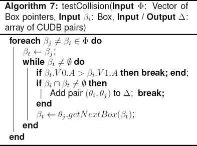
Figure 6 depicts the process for a 2D example with three objects. It shows the evolution of the variables used by the algorithm.

Fig. 6 2D example of collision 

6 CUDB Performance

CUDB has been compared with OUDB in number of elements and computation time for conversion to and from EVM and CCL (using OUDB-extended version [⁵]). The test datasets consists of 12 objects (see Fig. 7). All datasets come from public volume repositories, where from (g) to (l) are real volume models coming from CT or MRI scanners. The corresponding programs have been written in C++ and tested on a PC Intel R Core i7-4600M CPU@2.90GHz with 7.6 GB RAM and running Linux.

Fig. 7 Rendered images of the test datasets 

Table 1 shows the attributes of test datasets. For each dataset it shows size in voxels, number of foreground voxels (|F voxels|), number of triangles of a triangular surface mesh obtained via marching cubes [³⁶], number of extreme vertices (|EV |), number of boxes in its XYZ-OUDB (|OUDB|) and XYZ-CUDB (|CUDB|) representation, ratio between |OUDB| and |CUDB|, and number of connected components (|CC|) allowing non-manifold configurations.

Table 1 Attributes of the test datasets 

Note in this table that, although the number of boxes depends on the ABC-sorting of the original EVM, CUDB produces less elements than the other representations in all cases, regarding OUDB in some of the dataset less than 10% of elements. For instance, the XYZ-CUDB representation of the Lines dataset has only 3.8% of boxes of the corresponding XYZ-OUDB representation (see Fig. 8).

Fig. 8 Zoom in of Lines dataset. (a) XYZ-OUDB. (b) XYZ-CUDB 

Table 2 shows the performance of CUDB regarding OUDB. For each dataset it shows the time for: EVM to OUDB (E → O) conversion, OUDB-CCL (O_CCL), EVM to CUDB (E → C) conversion and CUDB-CCL (C_CCL). The last columns mean t_O = E → O + O_CCL, t_C = E → C + C_CCL, and the ratio between t_O and t_C.

Table 2 OUDB and CUDB run time comparison in milliseconds 

Note that, although the conversion from EVM to CUDB is slightly slower than EVM to OUDB due to the extra effort to merge the boxes, the CUDB-based CCL process is much faster due to the less number of elements and that we avoid the use of a equivalence table, in all datasets more than an order of magnitude, even the temple dataset more than two orders of magnitude faster. In any case, when computing the number of connected components starting from the EVM model, CUDB is more efficient than OUDB..

In order to show the performance of the CUDB-based exact collision detection, three scenes are presented. The first one consists of seven datasets (see Fig. 9), where the size of each is around 256³. The second scene consists of 250 spheres and 250 objects of the Star dataset randomly placed in a volume of 1000³ voxels (see Fig. 10). The third scene consists of 2 objects of the Cart dataset that have interlaced parts but do not collide (see Fig. 11).

Fig. 9 Collision scene 1. Six datasets: Armadillo (18338 boxes), Bunny (23410 b.), Cup (15002 b.), Dragon (19413 b.), FanDisk (4719 b.), Robot (3832 b.). In red the objects that collide: Bunny with Cup and Armadillo, and the latter with Robot 

Fig. 10 Collision scene 2. 250 spheres (voxel size 50×50×50) and 250 objects of the Star dataset (70×95×70). Each sphere has 907 boxes and each Star 1280 boxes in their corresponding XYZ-CUDB representation. In red the objects that collide 

Fig. 11 Collision scene 3. 2 objects of the Cart dataset. The original Cart has 100358 boxes, the rotated one 101743 boxes. Both in its XYZ-CUDB. The objects actually do not collide 

Statistics of the collision detection test are shown in Table 3. For each scene: number of objects (n), number of boxes of the object having the maximum number of boxes (m), total number of boxes in the scene (T), number of detected collisions (i.e., number of object pairs |pairs|) and time to detect the collisions in milliseconds.

Table 3 Statistics of the collision scenes 

Note that, although scene 3 has less boxes than scene 2, the required time for collision detection is bigger. This is because there is any collision, which implies that there is not any early discarding and all boxes must be evaluated.

7 Conclusion and Future Work

We have presented in detail, a new decomposition model for OPP, CUDB, which is an improved version of the OUDB model. Algorithms for conversion to and from EVM, for CCL and exact collision detection have also been presented.

Experimental results show that CUDB is smaller in number of elements, and so in storage size. It can be observed that computation of CCL is notably faster in CUDB than the improved version, OUDB-extended. Regarding the presented exact collision detection algorithm, although this is CPU-based, it is efficient when exact collision detection is required directly on CUDB models.

Table 4 resumes the pros and cons of CUDB with respect B-Rep and the hierarchical structures (HS) on the basis of some properties of solid representation schemes, and the CCL and collision detection performance.

Table 4 Comparative of CUDB vs. other representation models 

The performance variability of the presented algorithms is caused by the dataset size but above all to their surface intricacy. Our method depends on the number of boxes, tightly related to the model’s tortuosity (a property that represents the twist of a curve, i.e. the degree of turns or detours a model has [²⁶], like the previous developed methods based on OPP.

Characteristics of CUDB model have been exploited in some applications as in a CUDB-based virtual porosimeter [⁴⁴], which simulate mercury intrusion at increasing pressures, like the porosimeter lab. Also in a method to compute the Euler characteristic and the genus of binary volumes [¹⁴]. And a 2D version of the collision detection algorithm has been applied in a lossless simplification method to get a better shape preservation [¹⁵].

As future work, we are devising methods to compute the B-Rep model from the CUDB-representation and to obtain the CUDB-represented complement. Another future work is a complete analysis of whether any of the six ABC-sortings in CUDB produces an optimal number of disjoint boxes that cover the OPP, otherwise, one could think of allowing overlapping boxes in order to further reduce this number.

Finally, we think that CUDB model can be used to compute structural parameters of biomaterials as those reported in [⁶] and [⁵⁴] and new ones emerging in the bioengineering field.