1 Introduction

MЕМS vibratory gyroscopes as a part of Coriolis vibratory gyroscopes (CVG) are nowadays the most applicable in the modern industry and are intensively developing in the laboratories all over the world. The range of their applications is spreading from automotive to medicine including their traditional applications in aerospace. MEMS CVG technology compared to non-MEMS ones is attractive due to its capability to mass production and as a consequence to low cost.

Digital vibratory gyroscope including MEMS consists of three components: micromechanical component - sensing element, electronic component - dedicated electronics and software component - program implementing information processing and standing wave control algorithms. MEMS gyros differ from others by their sensing element that is manufactured by using surface and bulk micromachining technologies [²⁰, ¹⁷, ³, ¹²], such as film deposition, wet and dry etching, plating and others. MEMS structure design process is very complicated and time consuming, therefore there are some commercial MEMS CADs like Coventor Ware [⁸], Intellisuite [⁹] and others which facilitate and accelerate design process and analysis of vibrating microstructure.

This modeling using MEMS CADs can be called modeling at a micro-level. The result of micro-level modeling is a micro vibrating structure with certain geometrical and dynamic parameters. However, vibrating structure is not yet a gyro. In order to predict future gyro output characteristics modeling and simulation on the system level are required based on output parameters obtained at the micro-level modeling. MEMS gyro modeling at the system level consists of two sublevels: (1) electronic schematic and circuit board designs, (2) standing wave control and information processing algorithm modeling.

Digital gyro electronic hardware consists of analog, mixed and digital subcomponents. Analog subcomponent is usually called buffer that receives and amplifies analog signals from sensing element and filters signals before sending them to sensing element. Main elements of the mixed subcomponent are analog-to-digital (ADC) and digital-to-analog (DAC) converters.

Digital subcomponent is digital signal processing (DSP) system [²] or field programmable gate array (FPGA) with an auxiliary surrounding [¹⁰, ²²]. There are many CADs which facilitate and accelerate designing and simulation different types of electronic schemes and circuit boards. Some of them are SPICE, ProfiCAD, PCB123, EasyEDA, Ngspice, logisim, KTechLab and others. Many of them can be accessed in internet.

In order to model and simulate standing wave control and information processing algorithm mathworks Simulink is mainly used [¹¹, ¹⁹].

This paper is dealing with modeling, tuning and simulation of a standing wave control and information processing algorithm to show in detail how can be used the output parameters of micro-level modeling to obtain the output parameters of the future gyro. The considered here control and information processing algorithm will take into account low Q-factor of vibrating structure of preferably ring-type (such as micro fabricated ring, hemisphere, cylinder, and other bodies of rotation). Though considered here algorithms can control a standing wave of any MEMS or non-MEMS vibrating structures. As well-known there are two mode of CVG operation - rate and rate integrating ones [², ¹⁰, ¹¹, ¹⁹]. Investigations on differential mode of CVG operation have recently been appeared in the publications [⁴, ⁵, ⁶]. Differential mode of operation can effectively suppress external disturbances. All three modes of operations can be combined in single gyro to implement triple mode gyro [⁷] in contrast to dual mode gyro designed in [¹⁴].

In order to implement triple or dual mode gyro the algorithm should be represented in the form that allows one to switch from one mode to another without control program reloading. Most MEMS gyros operate in the rate mode. Rate mode algorithm is a simplest of three abovementioned, and the rate-integrating one is the most complex. In this paper the rate mode algorithm will be represented so that all three modes can be transformed from one to other by simple command of switching. Doing so the rate mode algorithm will obviously take more time for one iteration, than minimum possible, but in this case one can take advantage of switching to another mode swiftly without program reloading.

This paper presents operation principle of rate MEMS gyro on the example of ring resonator, detail description of the standing wave control algorithm operating in the rate mode, explanation of resonant frequency tracking principle built on the basis of digital phase lock loop (PLL), tuning of algorithm parameters such as drive and compensation signal’ phases and scale factor calibration bias dependence on resonator’s manufacturing imperfections.

2 MEMS CVG Principle of Operation

Let’s consider rate MEMS CVG operation principle using ring resonator. The primary standing wave is excited on the second resonant mode of the ring oscillations by applying periodical voltage U=Acos (ω_rt) with frequency ω_r close to the ring resonant frequency on drive electrode. Standing wave on the second resonant mode of the ring is characterized by four antinodes and four nodes of oscillations located along circumferential coordinate of the ring through the equal angles of 45 deg as depicted in the figure 1.

Fig. 1 Standing wave in a ring type MEMS CVG operation principle 

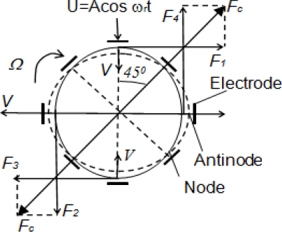
The solid and dashed ellipses in the figure 1 present the ring deformations in the first and second half of vibration period. When the resonator is rotating about its axis of symmetry (perpendicular to the ring’s plane) with angular rate Ω, Coriolis forces F₁, F₂, F₃ and F₄ arise, which excite secondary wave called Coriolis wave in the direction of resultant Coriolis force F_c directed under angle 45 deg relative to the direction of the drive force. The resultant Coriolis force is determined from the following relationship:

, (1)

where k is called an angular gain factor (Brian coefficient) depending on resonator geometry, V is linear velocity of ring’s mass points during vibration, α_v,Ω is an angle between vector V and vector Ω. As can be seen from the figure 1 α_v,Ω=π/2.

Linear velocity V of the ring’s mass points is:

, (2)

where µ₁ is transformation coefficient of applied to resonator voltage, U, and responded mechanical deformation.

Substituting (2) into (1) one can obtain:

. (3)

Thus, Coriolis force is proportional to angle rate Ω.

As can be seen from (3) Coriolis force F_c is changing with resonant frequency ω_r and its amplitude is proportional to angle rate. This means that sensing element output signal is amplitude modulated one. The resonant frequency is a carrier signal and angle rate Ω is a modulating signal. In order to obtain angle rate demodulation procedure should be applied to signal (3). Mechanical force F_c causes ring’s deformation with amplitude proportional to this force. Sense electrode, located under the angle of 45 deg to drive one, transforms mechanical amplitude into electric signal U_c= µ₂F_c, where µ₂ is transformation coefficient of mechanical deformation into responded voltage U_c. Then, electric signal U_c is demodulated to obtain signal proportional to angle rate:

, (4)

where SF is a gyro scale factor known as a result of calibration using rotating table.

In order to increase gyro bandwidth that allows one to measure fast changing angle rate force-to-rebalance method of measurement is used [¹⁵].

In the force-to-rebalance measurement method the signal U_c is driven to zero with the aid of feedback control system. The signal that compensates to zero for the Coriolis force is proportional to angle rate.

MEMS CVG can also operate as a rate-integrating (whole-angle mode) gyro [¹⁵] at which Coriolis force is not compensated for. In a rate-integrating gyro standing wave freely rotates under action of Coriolis force. In this case standing wave angle of rotation is proportional to gyro angle of rotation and coefficient of proportionality is angular gain factor k (Brian coefficient).

Returning to the rate MEMS it should be noted that parameters A and ω_r in SF expression (4) should be stabilized to make SF constant. But ω_r (resonant frequency) is changing versus temperature during operation and under environment temperature changes, so this parameter should be tracked and measured. Vibration amplitude should be stabilized at prescribed value A₀ during angle rate measurements. Besides, quadrature (error) signal that arises due to manufacturing imperfections and Coriolis force should be nulled to implement force-to-rebalance method of measurement. So, four control systems should be implemented to accurately measure angle rate by MEMS gyro.

In order to implement all four above mentioned control circuits, eight diametrically connected electrodes, shown in figure 1, should be used. So, there are only four independent electrodes, two of them are used to apply control signals on sensing element, specifically, to drive primary vibration and to compensate for the Coriolis force, and another two which are used to sense the responded signals.

3 MEMS Gyro Dynamic Equations

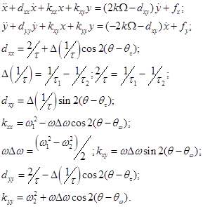
In order to model MEMS gyro, first of all sensing element dynamic equations with real errors resulting from manufacturing imperfections should be accepted. There are well-known dynamic equations (5) of two dimensional pendulum [¹⁵] that fit our aim. Equation parameters explanations are presented in figure 2.

Fig. 2 Rigidity and damping axes 

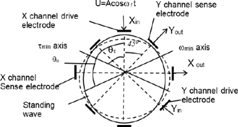
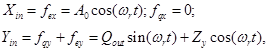
In these equations k is Brian coefficient, d_xx is the X axis damping coefficient, τ₁ is a minimum resonator’s damping time, τ₂ is a maximum resonator’s damping time, d_xy is a damping cross-coupling coefficient, k_xx is a normalized by mass resonator rigidity along the X axis, ω₁ and ω₂ are maximum and minimum resonant frequencies, k_xy is a rigidity cross-coupling coefficient, d_yy is the Y axis damping coefficient, k_yy is a normalized by mass resonator rigidity along the Y axis, f_x, f_y are normalized by mass control signals, θ_ω is an angle between minimum frequency axis and standing wave (antinode) axis, θ_τ is an angle between minimum damping axis and standing wave axis:

(5)

Variables x, y, f_x and f_y in equations (5) correspond to variables X_out, Y_out, X_in and Y_in presented in figure 2, respectively. In these designations X_out and Y_out are sense signals, i.e. displacement of resonator’s mass point from its initial static position expressed in voltages, and X_in and Y_in are control signals. System of equations (5) is valid to describe any type of resonator, not only ring type.

In the rate mode of CVG operation standing wave is immovable relative to resonator. They are rotate together with the same angle rate. In this case angle θ between direction of vibration and direction of drive force (X_in axis) is constant and equal to zero. MEMS sensing element as shown in figure 2 can be interpreted as a two-input-two-output plant. The model of the MEMS resonator based on (5) is presented in figure 3 in designations of Simulink blocks.

Fig. 3 MEMS sensing element model based on equations (5)  

Full schematic in the right side of figure 3 (called sensing element) is presented as a subsystem that has four input and two output signals.

Primary standing wave drive signal, f_x, Coriolis force compensation signal f_y, input angle rate signal, Om, that should be measured and θ (teta in figure 3) signal which is equal to zero for rate mode of MEMS operation.

As discussed above we will present the standing wave control algorithm in such modification that allows one to change the modes of MEMS operation by simple switching without processor’s program reloading. In rate integrating mode of operation standing wave angle θ is changed. This angle θ during simulation should be calculated and sent it to the sensing element model to change the position of standing wave as it is in the real resonator, but in this paper angle θ=0, because rate mode of MEMS gyro operation is only considered.

Upper schematic of figure 3 represents the model of the first equation of system (5) in designations of the Simulink blocks. The second equation of system (5) model has not shown in the figure 3 because it is similar to the first one. The central schematic shows combination of the two equation models with possibility to introduce sensing element parameters like Q-factor, resonant frequency, frequency mismatch, Q-factor mismatch, and angular dispositions of minimums of damping θ_τ and rigidity θ_ω axes. These parameters mainly determine resonator’s manufacturing imperfections and gyro accuracy.

4 Rate MEMS Digital Control System

MEMS CVG control system block diagram is presented in figure 4. The standing wave is excited at the resonant frequency ω_r of the second mode of ring vibrations. Drive wave control is based on two subsystems: phase lock loop (PLL) and automatic gain control (AGC).

Fig. 4 CVG control system block diagram operating in rate mode of operation 

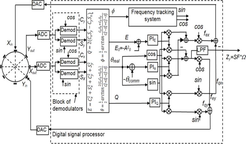
These two subsystems generate drive signal Xin(t) of proper amplitude, frequency and phase to sustain primary vibration in changing environmental conditions. PLL provides resonant frequency tracking when it changes and AGC keeps the primary vibration amplitude at the constant desired amplitude A₀.It should be noted that all signals coming from resonator are amplitude modulated ones.

The resonant frequency is a carrier frequency and angle rate Ω is modulating signal. In order to calculate control signals, first of all demodulation should be carried out. In order to apply control signals to the resonator, re-modulation using resonant frequency should be carried out.At gyro rotation there appears at Y_out electrode secondary vibration signal caused by Coriolis force together with error signal which is called quadrature, Q. These two signal components are separated by demodulation processes using reference signals generated by PLL.

Sine component amplitude is proportional to angle rate SF*Ω, and cosine component amplitude is a quadrature signal, which is an error caused by resonator manufacturing imperfections.

Then, these two signals are re-modulated, combined and sent to the Yin electrode as a compensation (force-to-rebalance) signal to keep the standing wave in stationary position relative to resonator.

The control system operates as follows. Antinode X_out and node Y_out signals after analog-to-digital converters (ADC) are splitting and provided to the block of demodulators where they demodulate with sine and cosine of resonant frequency as the reference signals to obtain four slow changing signal C_x, S_x, C_y, and S_y as shown in figure 4. In essence, C_x, S_x, C_y, and S_y signals can be used as control signals for rate MEMS gyro.

However, to implement so called “universal” algorithm that allows one, as discussed above, to switch from rate to rate-integrating and to differential modes of MEMS gyro operation without program reloading, these four signals C_x, S_x, C_y, and S_y are provided to block of pendulum variables (A₀)²=E, Q, θ, φ calculation.

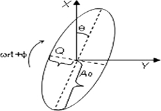
Physical interpretation of pendulum variables is presented in figure 5 [¹⁵], where trajectory of resonator point mass during vibration is shown. In the figure 5, A₀ is vibration amplitude, Q is quadrature amplitude, θ is a standing wave angle relative to X axis and φ is a vibration phase.

Fig. 5 Pendulum variables 

These pendulum variables can be calculated as follows [¹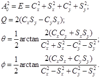⁶].

(6)

For rate MEMS gyro the pendulum variables should be retained at the following values Q=0, E=const, θ=0, φ=0.

These relationships can be implemented with the aid of four, one for each parameter, proportional and integral (PI) controllers. It should be noted that when: θ_comm=0 (see figure 4) MEMS gyro operates in the rate mode, when

MEMS gyro operates in the differential mode [⁴]. When connection between θ_r and PI_θ controller is opened, MEMS gyro operates in rate-integrating mode. Thus, it can be implemented triple mode MEMS gyro [⁷]. Dual mode CVG has been implemented in hemispherical resonator gyro (HRG) [¹⁴].

4.1 Demodulation

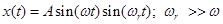
In the block of demodulators four identical synchronous demodulators are used to separate envelope from amplitude modulated signals both from X_out and Y_out with the aid of two reference signals sinω_rt and cosω_rt generated by PLL. Each demodulator consists of multiplication unit, low pass filter to suppress high frequency component, arising after multiplication, to separate low frequency envelope and to double it as depicted in figure 6 to obtain the envelop.

Fig. 6 Synchronous demodulator 

For example, let’s take amlitude modulated signal as follows:

, (7)

where Asin(ωt) is an envelope and sin(ω_rt) is a carrier. Graph of this function, for f_r=2πω_r=4 kHz, f=2πω=100 Hz and A=1, is presented in figure 7.

Fig. 7 Amplitude modulated signal 

After multiplication by reference signal sin(ω_rt), low pass filtering (LPF) and doubling, in accordance with block diagram shown in figure 6, the following output signal can be obtained:

(8)

4.2 Frequency Tracking System

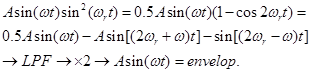
The idea of the resonant frequency tracking is based on the fact that the drive signal (X_in) and responded signal (X_out) in resonator have π/2 phase difference when drive signal frequency is equal to resonant one. When drive frequency defers from resonant one there appears addition ±φ to π/2 as shown in figure 8. This means that X_out signal has quadrature component which amplitude is proportional to φ and its sign indicates whether the drive frequency is more or less of resonant one. The basic component of X_out signal is used to control (stabilize) the vibration amplitude, and quadrature component is used to track the resonant frequency.

Fig. 8 Amplitude and phase frequency characteristics of resonator 

Really, let’s consider the typical resonator normalized amplitude-frequency (AFC) and phase-frequency (PFC) characteristics. From figure 8 follows that when the drive frequency is not equal to resonant frequency the phase of the X_out signal acquires additional phase ±φ.

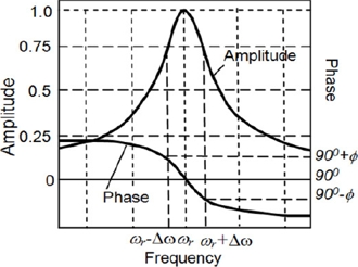
For example, let the drive signal is not at the resonant frequency X_in=Bcos((ω_r+∆ω)t), then the responded signal, in accordance with figure 8, is X_out=A₀sin(ω_rt-φ).

This means that to the sine component of X_out signal the cosine component is added. Cosine component of the X_out signal is extracted by the block of demodulators (see figure 4) which is proportional to the phase difference φ between reference signal cos(ω_rt) and X_out signal:

(9)

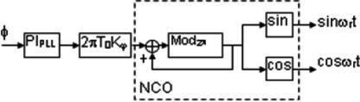
The signal proportional to phase difference φ, which is calculated by the last expression of (6), as an error signal is provided to proportional and integral PI_PLL controller which, after multiplication by sample time T₀ and amplification K_ϕ times changes the output frequency of numerically controlled oscillator (NCO) so that to null the error signal φ as shown in figure 9.

Fig. 9 Block diagram of the resonant frequency tracking system based on PLL 

For rate mode of MEMS operation (φ=0) is equivalent to C_x=0.

4.4 Standing Wave Angle Control

When θ_comm=0, PI_θ controller (see figure 4) generates such an output signal that drives to null the difference (θ_r - θ_comm) → 0, where θ_r is an actual standing wave angle and θ_comm is a commanded value of standing wave angle. When θ_r=0, drive X_in and compensation Y_in signals are:

(10)

where Q_out is an output signal of the PI_Q controller, and Z_y is a signal proportional to angle rate measured. Thus, X is a drive channel and Y is a measurement channel.

When: θ_comm=θ₀=const≠0,πk/4, k=1,2,…, i.e. standing wave angular position does not coincide with any of eight electrodes, there arise two X and Y measurement channels with opposite angle rates. The biases and scale factors of these two channels are dependent on angle θ₀. One can choose angle θ₀ such that biases of X and Y channels will be equal to each other, then the difference of the two channels increases angle rate and compensates for the bias in difference channel.

There is another option of choosing angle θ₀ such that scale factors of the two channels are equal to each other. In this case external disturbances acting on the gyro can be effectively compensated for in difference channel [⁴, ⁵]. There are also other advantages of differential mode of operation [⁶].

When connection between θ_r signal and PI_θ controller is opened MEMS gyro operates in rate-integrating (whole angle) mode. In this case standing wave freely rotates under action of Coriolis force and θ_r is output signal proportional to angle of gyro rotation.

5. Drive and Compensation Signal Phases Tuning

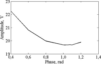
In the gyro model like in real gyro it is important to tune drive and compensation signal phases. Tuning criteria can be different. In this work to tune drive phase, criterion of minimum of drive signal amplitude providing desired vibration amplitude A₀ is chosen.

Figure 10 shows dependence of drive signal amplitude on its phase. From this figure one can see that this minimum is not sharp and permits variation in the vicinity of minimum point without significant change in amplitude. Thus, minimum amplitude is reached in the phase range [1-1.1] rad.

Fig. 10 Drive signal phase tuning 

In spite of that model output is dimensionless and in real digital MEMS gyro output signals are represented in digital code, it is advisable to normalize output signal of ADC such that output code would be numerically equal to the voltage on its input. It will be very convenient to visually analyze such digital signals. Therefore, output signals of the gyro model in this paper will be represented in volts.

In order to tune phase of compensation signal, minimum of module of angle rate in percent which is visible in the quadrature signal is chosen as a tuning criterion. Figure 11 shows the dependence of angle rate portion in percent which is visible in quadrature signal versus compensation signal phase.

Fig. 11 Compensation signal phase tuning 

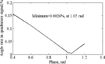
As can be seen from this figure minimum is reached at the phase value of 1.05 rad which is in the range of minimum of drive signal phase. It is interesting to note, that in real gyro drive and compensation signal phases are also close to each other. When compensation signal phase is more than 1.2 rad or less than 0.2 rad, then feedback control subsystem providing compensation for the Coriolis and quadrature signals becomes unstable. When these tunings are not properly accomplished, then the higher portion of input angle rate will be visible in the drive and quadrature signals that results in accuracy reduction or even instability.

6 Simulation Results

In order to start simulation let’s introduce a noise in the model to make the model close to real gyro. The noise can be introduced on the output of ADC with such standard deviation that the output angle rate signal noise would be close to known MEMS gyro, for example, one of the gyro from the block of sensors ADIS16367 (Analog Devices, USA).

Gyro model operates at sampling frequency 50 kHz and output LPF has cutting frequency 300 Hz. Besides, gyro model scale factor calibration should be made before the beginning of simulation, like it occurs in real gyro. After that, the output signal proportional to angle rate measured should be divided by scale factor to obtain angle rate in deg/s.

Usually, scale factor (SF) calibration is conducted for some different angle rates from the gyro measurement range, and then, these scale factor values are averaged to reduce errors from SF nonlinearity. We simplify this procedure and conduct gyro model SF calibration at one value of angle rate equal to 100 deg/s. For this purpose, in accordance with international IEEE standard [¹⁵], it is necessary to rotate the gyro clock-wise and counter-clock-wise with equal angle rates of Ω_r=±100 deg/s, then, mean values of measurements Np and Nm are calculated for each direction of rotation, and then, SF is calculated by the formula:

. (11)

Figure 12 shows noisy output signal of the gyro model under clock-wise and counter-clock-wise rotation with Ω_r=±100 deg/s with indication of mean values N_p and N_m. Calculation shows that SF=0.03241 V/(deg/s).

Fig. 12 Scale factor and bias measurement during rotation 

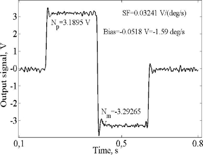
Because gyro model (and real digital gyro) output signal is represented in digital code numerically equal to voltage on the input of ADC, as we discussed above, SF dimension can also be represented in 1/(deg/s). Using the same measurements, N_p and N_m, gyro bias, B, during rotation can be calculated as follows:

. (12)

After scale factor determination, rate MEMS gyro model output signal will be presented in deg/s.

It should be noted that rate MEMS gyro bias depends on resonator parameters imperfections, and SF linearly depends on resonant frequency and vibration amplitude (4). Bias and SF have been obtained at the following resonator parameters:

Figure 13 shows dependence of bias on frequency mismatch expressed in percent (∆f/f)*100%. Negative percent means that axes of maximum and minimum resonant frequency exchanged their positions.

Fig. 13 Bias versus frequency mismatch 

As can be seen frequency mismatch significantly affects bias and this dependence is close to parabola. This graph says that bias is very sensitive to frequency mismatch. This sensitivity is about 130 deg/s/%. So, frequency mismatch should be made close to zero. In order to make frequency mismatch close to zero in real MEMS gyro electrostatic stiffness tuning [²¹] or laser trimming [²²] can be used.

Figure 14 shows dependence of bias on Q-factor mismatch expressed in percent, (∆Q/Q)*100%.

Fig. 14 Bias versus Q-factor mismatch, ∆Q/Q 

In contrast to figure 13 Q-factor mismatch influences on bias non-symmetrically and has much lower sensitivity of about 0.03 deg/s/%, than that of frequency mismatch.

Figure 15 shows bias dependence on θω angle.

Fig. 15 Bias versus θω angle 

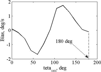
This dependence is close to harmonic with two periods on full revolution.

Closer to harmonic one is the dependence of bias on θτ angle shown in figure 16.

Fig. 16 Bias versus θτ angle 

This figure shows that bias sensitivity to θ_τ angle is much lower with the maximum value of about 1.4×10^-3 (deg/s)/deg in contrast to bias sensitivity to θ_ω with the maximum value of about 3×10^-2 (deg/s)/deg.

From the data presented in figures 15 and 16 follows that by forced rotation of a standing wave, through the angle 90 deg, change of a gyro bias, caused by frequency and Q-factor mismatches, can be compensated for.

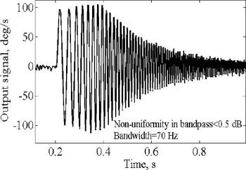
Figure 17 shows gyro model output signal when input angle rate changes its frequency from DC to 200 Hz. This figure shows bandwidth of the gyro model on the level of 70 Hz, and non-uniformity in band pass of no more than 5%. SF does not depend on the considered here parameters. Gyro model and real gyro SF linearly depends on amplitude of vibration and resonant frequency. SF sensitivity to resonant frequency is much less than that of vibration amplitude.

Fig. 17 Model gyro bandwidth determination 

7 Conclusion

This paper presents MEMS gyro model based on “universal” algorithm enables implementing any of three modes of MEMS operation - rate, rate-integrating and differential ones. Also, this gyro model gives opportunity to implement new triple mode MEMS gyro.

Using this MEMS gyro model tuning procedure has been shown. Dependences of bias on orientation angle θ_ω of rigidity and angle θ_τ of damping axes have been obtained. Based on these dependences maximum value of bias sensitivities to such resonator imperfections as frequency, Q-factor mismatches, θ_ω and θ_τ angles have been determined. It was found out that gyro bias can be compensated for by forced rotation of standing wave through the angle 90 deg.

This rate MEMS gyro model can be used to investigate influence of shock and vibration on the output signal in order to estimate gyro sensitivity to them.

Moreover, presented in this paper gyro model can help developer to implement rate-integrating (whole angle) and differential modes of MEMS operation, investigate their sensitivity to different types of internal and external disturbances.

In this paper PI controllers are used to provide necessary bandwidths for the MEMS gyro control subsystems. In order to improve MEMS gyro control in harsh environment robust PID tuning [¹³], adaptive PID, fuzzy logic, sliding mode [¹] and their combinations can be used.