


 nueva página del texto (beta)
 Inglés (pdf)
 Artículo en XML
 Referencias del artículo
 Enviar artículo por email
 Citado por SciELO
  Similares en
SciELO
Similares en
SciELO 
 Permalink
1 Introduction
The Particle Swarm Optimization (PSO) algorithm was originally proposed by Kennedy and Eberhart in the mid-1990s 10, 6. PSO is a population-based stochastic search algorithm whose original aim was to solve continuous optimization problems. The members of the population are called particles in PSO, and they are represented in vectorial form by their position x in the search space. A particle also stores the position p (its personal best) with the best fitness value that this particular particle has reached so far. The particles change their position through a process that incorporates a velocity. Such a velocity is computed using the personal best position p of the particle and the position g of the particle with the best known fitness value of the swarm (called the global best). The formula to compute the velocity is shown in Equation (1):
The current velocity υt+1 is computed by adding two components to the previous velocity υt of the particle. The first component is the difference between the current position x of the particle and the position p with the best value obtained by the particle. This is called the cognitive component. The second component is computed by the difference between the current position x of the particle and the position g of the best known value of all particles of the swarm. This is called the social component. The components are multiplied by the learning constants c1 and c2. Usually the value of these constants is the same, and greater than one. Each component is also multiplied by random numbers r1 and r2, respectively. Using this computed velocity, the next position of the particle is updated using Equation (2):
One of the keys for the popularity of the PSO algorithm is its simplicity, since, as shown before, it consists only of two equations to update the position of the particles.
2 Velocity Regulation
The regulation of the velocity has been important since the initial developments of the PSO algorithm; Eberhart 6 discussed the use of a maximum value for the velocity, and showed results for different values of the maximum velocity. A more complete study on the effects of the velocity limit is shown in 9 by Kennedy and later in 11, where Shiand Eberhart introduced the Inertia Weight method (IW) to limit the velocity of the particles. The IW method consists in multiplying a factor w called inertia to the previous velocity of the particle when the current velocity is computed, thus Equation (1) is rewritten as:
In order to balance global and local search, the inertia factor w is introduced. In 11, the authors also used a maximum velocity value. They also tested several values for the inertia weight in order to determine which of them produced better results. In a further paper (see 12) a linear decreasing value for the inertia weight factor w, is proposed. In this case, the authors also limited the maximum value of the velocity. Shi and Eberhart 12 also proposed to use the maximum value of the position as a limit to the velocity, and thus the maximum values for the velocity, for dimension i are (-Vi-max , Vi-max ) with Vi-max = Xi-max .
The second most popular method to regulate the velocity is the constriction factor, which was originally introduced by Eberhart 7, and is discussed in detail in 5. This method also consists in multiplying a factor not only to the last computed velocity but to the full computed velocity as expressed in Equation (4):
The constriction factor is computed as a function of the learning constants as shown in Equation (5)
where φ is the sum of the learning constants φ = c1 + c2, and k is an arbitrary constant in the range [0,1]. Eberhart 7 recommended as a rule of thumb, to use a velocity limit along with the constriction factor method. Bratton and Kennedy 4 defined a standard PSO algorithm (SPSO), for which it was suggested the use of a local ring topology. In SPSO a particle can only communicate with a limited number of particles (typically, with only two other particles) and not with the full swarm. The Constriction Factor model uses a swarm size of 50 particles, with a non-uniform initialization of their positions. Additionally, this approach allows the particles to leave the feasible search space, but when that happens it does not evaluate the best position of such infeasible particles. This approach does not include a limit to the velocity but recommends the use of a generous Vmax value. Thus, although the aim of the inertia weight and the constrictor factor methods is to achieve a balance between exploration and exploitation, it also attempts to limit the particles' velocity. In order to avoid that the particles stray far away from the boundaries of the search space, the use of an explicit velocity limit is recommended. Other research works 8 try to adapt or modify the value of w, but they do not discard the use of a factor to limit the velocity.
Barrera and Coello 3 proposed a version of the PSO algorithm without the use of the Inertia Weight factor or Constriction model, but introduced a parameter r ∈ (0,1). A factor rt is used to compute a new velocity limit, as show in the following equation:
where lit is the velocity limit for the ith variable at iteration number t, and is the initial velocity limit for the ith variable.
In a more recent work, Adewumi and Ara-somwan 1 presented the Improved Original PSO (IOPSO) with dynamic adjusted velocity and position limits. The velocity limits for each variable are computed in this case as a fraction of the current limit for the position. Thus, the maximum and minimum velocities for the ith particle are computed using the following equations:
where xmin and xmax are the minimum and maximum values for the position of a particle, respectively.
The values for xmin and xmax are computed at each iteration by finding the minimum and maximum values for all variables of all particles. This is done by first computing the upper and lower bounds Ld and Sd:
where
Thus, the value of the velocity limit is changed dynamically as the values for xmax and xmin change.
Here, we propose a method that only uses the velocity limit. We argue that our proposed approach is simpler than the existing ones, since it does not use any factor to alter the particle's velocity. In fact, our proposed approach somehow provides a simplified version of the PSO algorithm, since it eliminates the use of the learning constants.
3 Velocity Limit Decreasing Method
In order to have a good balance between exploration and exploitation by only using a velocity limit, the limit of the velocity is changed at every iteration of the PSO algorithm. To do this, the velocity limit Li for the ith variable is initialized to half of the length of its search limits, as defined in Equation (7):
Then, at each iteration, to compute the current velocity limit li(t), the initial velocity limit Li is multiplied by a factor which is a function of the current iteration t. Therefore, the limit for the velocity at iteration t is:
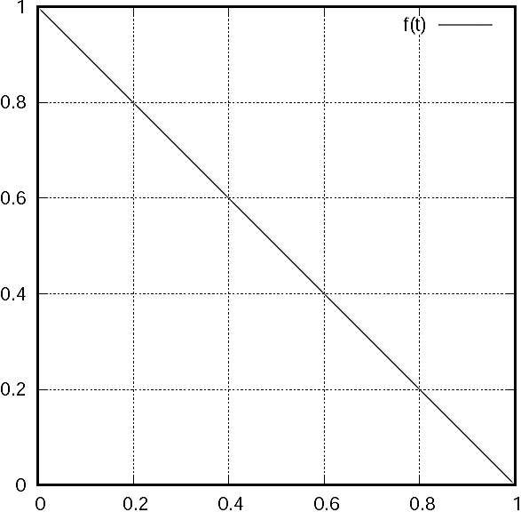
where f(t) is a given function. The simplest case to test is a simple straight line, as defined in Equation (9):
The plot of the function f(t) is shown in Figure 1. The function in Equation (9) is defined in the range [0, 1] and returns values in the same range. For the initial value t = 0, f(0) = 1, and for the last value, t = 1, we have f(1) = 0. In order to use the function of Equation (8), we divide the current iteration by the total number of iterations. The velocity limit at iteration t is computed using:
where tmax is the total number of iterations. The idea is that gradually decreasing the velocity limit helps the swarm to converge at the end of the evolutionary process but, at the same time, it allows the particles to explore the search space at the beginning. Equation (10) can be adjusted if the termination criteria is a maximum number of function evaluations emax instead of a given number of iterations. Equation (10) is written as follows:
where e is the current number of function evaluations and emax is the maximum number of evaluations.
Contrasting with the work of Barrera and Coello 3, we present here a more general method. Setting the function f(t) in Equation (8):
for a certain fixed value of r, it produces the method described in 3. Function f(t) can be modified to use more parameters, although our goal is to have a simpler version of the PSO algorithm. We avoid adding any extra computations or dependencies. We also avoid limiting the position of the particles. Unlike the method proposed by Adewumiand Arasomwan 1, we do not modify the position of the particles if they go out of the feasible space. Thus, we have less extra computations. Additionally, the particles out of range are not evaluated in order to avoid performing unnecessary function evaluations.
A simple linearly decreasing velocity limit may result in an equilibrium between local and global search, but we aim to give PSO the capability to perform global search for a longer time or to achieve a faster convergence. We explored the use of polynomial functions to regulate the form the velocity limit decreases with time.
We used the following set of functions to try to enhance the global search over the local one:
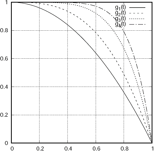
The g functions are derived from the simplest non-linear function, the parabola g(x) = x2. Close to the value x = 0 the function is evaluated to g(0) = 0 and for x = 1 we have g(1) = 1. Thus, g(x) is a good candidate to be used as our f(t). The parabola function is easily transformed first by a reflection in the x-axis by multiplying by -1 with the result g0(x) = -x2 and values g0(x = 0) = 0, and g0(x = 1) = -1. Finally, we add 1 to get the required values for the function f(t). That is, we have g1(x) = -x2 + 1 with values g1(x = 0) = 1 and g1(x = 1) = 0. The rest of the g functions are obtained using a similar method, but increasing the power of the variable being evaluated. This gives us the result of a slower decrease at the values close to t = 0 and a faster decrease at the values close to t = 1.
The change in the power of the variable t gives flexibility in the adjustment of how the velocity limit decreases. It is also possible to use fractions in the power value to have a function f(t) close to the behavior of a straight line.
Those functions decrease more slowly in the values closer to zero, and decrease faster as their argument is closer to one. As we increment the value of the power of x, the longer is the effect of a slow decrement. Conversely, the decrement is faster as the argument is closer to one. The plot of the g functions is shown in Figure 2.
On the other hand, in order to enhance the use of local search over the global search, we used the set of functions h, described in equations (17-20):
The plot of the h functions is shown in Figure 3. The h functions in contrast to the g functions, decrease faster if their argument is close to zero, and more slowly as it approximates to one. The h functions are derived with a similar method as the g functions, and from the same base function, the parabola. In this case, a reflection is not needed but a displacement of the position where the parabola evaluates to zero. This is done by subtracting 1 from the variable, so we have h0(x) = (x-1)2, and no further modification is needed since h0(x = 0) = 1 and h0(x = 1) = 0. Thus, we set h1(t) = (t - 1)2. In this case, it is necessary to be careful if we raise the value of the power. For the odd values 3, 5, 7 a reflection in the x-axis is needed to achieve the desired results.
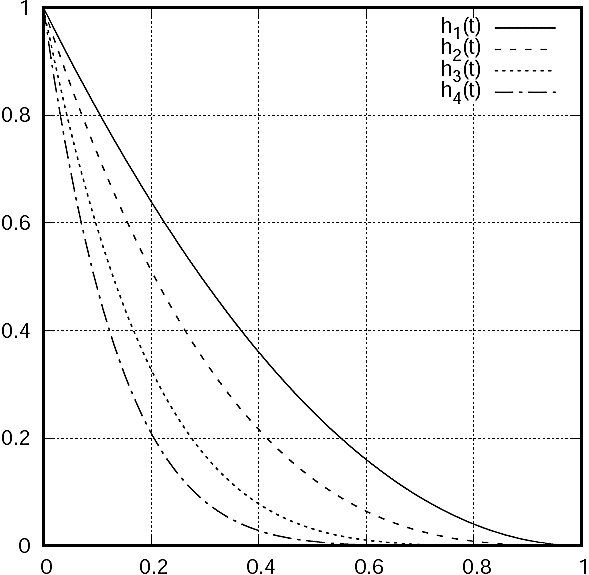
Fig. 3 The set of functions h. These functions decrease faster as they approach zero and they decrease more slowly as they approach one
Using the functions described above, we start with a velocity limit of Li and then decrease the limit, slowly at the beginning and faster at the end, for the set of functions g, and faster at the beginning and slower at the end for the set of functions h. An alternative strategy is to start with a small value for the velocity limit li , increase to a maximum, and then finally decrease it again. In order to achieve this, we use the functions l and m which are defined in equations (21) and (22), respectively:
The plot of function l is shown in Figure 4. The function is a parabola adjusted to have values of zero at the positions t = 0 and t = 1 and to have a maximum value of one in the position t = 0.5. Function l increases and decreases fast.
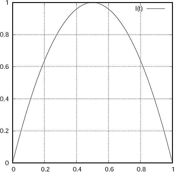
Fig. 4 The function l. This function starts with a small value and it increases and then decreases slowly
The plot of function m is shown in Figure 5. Function m is a composition of two parabolas adjusted to have values of zero at t = 0 and t = 1 and have a maximum value of one at t = 0.5. The function m increases and decreases slower than function l.
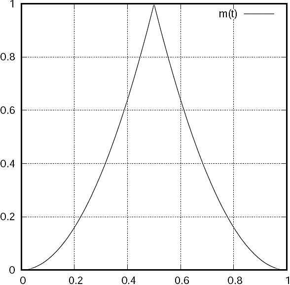
Fig. 5 The function m. This functions starts with a small value and it increases and then decreases fast
We do not make any change to the original equations for computing the position and velocity of a particle. Thus, we use the following equations to compute them:
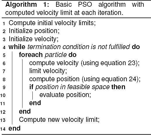
The algorithm for our version of the PSO algorithm is outlined in Algorithm 1. The only change in the algorithm, with respect to the original PSO, is the computation of the velocity limit for the current iteration or function evaluation count (lines 1 and 13).
4 Experiments and Results
The PSO algorithm used in the experiments is presented in Algorithm 1, where the initialization of the position of the particles is asymmetric (only in a region of the search space). The topology adopted is the global best (gbest), that is, the best position g is selected from all particles in the swarm. If a particle leaves the feasible space, its position is not updated, i.e., the position and velocity of the particle are not modified. The iteration of the PSO algorithm ends when the maximum number of function evaluations is reached. The reported results are the numeric error computed as |f(x) - f(x*)|, where f(x) is the best value obtained after the termination criteria is reached, and f(x*) is the value of the optimum of the test function being evaluated.
The parameters used in the experiments are the same as those adopted in 4. Such parameters include a swarm size of 50, a number of 300,000 function evaluations, and 30 dimensions for the n-dimensional test functions. The inertia weight is w = 0.729 and the learning constants are c1 = c2 = 1.49445. The initialization of the position of the particles is asymmetric 2, and 30 independent runs were performed to collect our statistics. In the following sections we present a comparison of the results obtained with the standard PSO and using the described functions to decrease the velocity limit with the description of the obtained results.
4.1 Standard PSO and Linear Decreasing Velocity Limit
The first experiment is to use the linear function described in Equation (9) to decrease the velocity limit (see Figure 1). Results for the comparison of the standard PSO versus the linear decreasing limit, mean value only, are shown in Table 1.
Table 1 Comparison of the results of the standard PSO and the linear decreasing velocity limit
| Function | standard PSO | Linear decreasing |
| mean | mean | |
| ackley | 1.9733E+01 | 1.9980E+00 |
| camelback | 4.6510E-08 | 9.8186E-06 |
| goldsteinprice | 2.4300E+01 | 4.7737E-05 |
| griewank | 1.7208E-02 | 1.0668E+00 |
| penalizedone | 1.2097E-01 | 2.9167E-01 |
| penalizedtwo | 4.6242E-02 | 3.8737E-01 |
| rastrigin | 1.7113E+02 | 6.3297E+01 |
| rosenbrock | 4.4084E+01 | 4.1856E+02 |
| schwefelone | 1.8303E+01 | 5.7644E+02 |
| schwefeltwo | 1.6349E+04 | 1.7797E+04 |
| shekelfive | 5.0524E+00 | 5.0534E+00 |
| shekelseven | 5.2741E+00 | 4.9237E+00 |
| shelelten | 5.3608E+00 | 5.3616E+00 |
| sphere | 2.0311E-18 | 7.7532E+00 |
From Table 1, we can observe that in three test functions the method of linearly decreasing the velocity limit produced better results. In the other test functions, the results are comparable, although in the case of the Sphere, we obtained a worse result than the standard PSO.
4.2 Balancing Exploration and Exploitation
To try to balance exploration and exploitation, we used second order polynomials to limit the velocity. Such polynomials are described in equations (1316) and they decrease first slowly and then fast. We expect this to help the exploration phase of the PSO algorithm. Conversely, the polynomials described in equations (17-20), which decrease first fast and then slower, are aimed to foster the exploitation phase.
The results of the g family function are shown in Table 2. The first column corresponds to the test function being used. The second column contains the mean value for the standard PSO (SPSO) and the rest of the columns show the mean values for the g function family. The results in Table 2 show than in some cases we have better results but this is not the general case. The results for the Sphere test function are worse than those obtained from the simple linear decrease of the velocity limit.
Table 2 Comparison of the results of the standard PSO and the g family function
| Function | SPSO | g1 | g2 |
| mean | mean | mean | |
| ackley | 1.9733E+01 | 2.9982E+00 | 3.6223E+00 |
| camelback | 4.6510E-08 | 5.8372E-05 | 1.1289E-04 |
| goldsteinprice | 2.4300E+01 | 3.5533E-04 | 5.1748E-04 |
| griewank | 1.7208E-02 | 1.2698E+00 | 1.6192E+00 |
| penalizedone | 1.2097E-01 | 1.1242E+00 | 2.3880E+00 |
| penalizedtwo | 4.6242E-02 | 1.7024E+00 | 4.3971E+00 |
| rastrigin | 1.7113E+02 | 9.4992E+01 | 1.4980E+02 |
| rosenbrock | 4.4084E+01 | 1.0466E+03 | 3.4962E+03 |
| schwefelone | 1.8303E+01 | 1.4625E+03 | 2.0464E+03 |
| schwefeltwo | 1.6349E+04 | 1.8399E+04 | 1.8819E+04 |
| shekelfive | 5.0524E+00 | 4.2201E+00 | 3.4036E+00 |
| shekelseven | 5.2741E+00 | 4.2305E+00 | 4.2445E+00 |
| shelelten | 5.3608E+00 | 4.4778E+00 | 4.1323E+00 |
| sphere | 2.0311E-18 | 3.3257E+01 | 6.9510E+01 |
| Function | g3 | g4 | |
| mean | mean | ||
| ackley | 4.7230E+00 | 5.6539E+00 | |
| camelback | 2.2151E-04 | 4.1503E-04 | |
| goldsteinprice | 1.9029E-03 | 1.6954E-03 | |
| griewank | 2.6719E+00 | 4.1273E+00 | |
| penalizedone | 5.1595E+00 | 8.7892E+00 | |
| penalizedtwo | 1.7640E+01 | 1.1807E+02 | |
| rastrigin | 1.7465E+02 | 1.9648E+02 | |
| rosenbrock | 9.1464E+03 | 2.2028E+04 | |
| schwefelone | 3.0486E+03 | 3.8498E+03 | |
| schwefeltwo | 1.9409E+04 | 1.9721E+04 | |
| shekelfive | 3.8006E+00 | 3.9139E+00 | |
| shekelseven | 3.9175E+00 | 3.4235E+00 | |
| shelelten | 3.3001E+00 | 3.9070E+00 | |
| sphere | 1.7368E+02 | 3.4825E+02 | |
Next, we test the h family functions. With this family of functions, we expect to favor the exploitation phase of the PSO algorithm. Table 3 shows the results for the h family of test functions. The results follow the same order as that in Table 2.
Table 3 Comparison of the results of the standard PSO and the h family function
| Function | SPSO | h1 | h2 |
| mean | mean | mean | |
| ackley | 1.9733E+01 | 8.3318E-02 | 1.2198E-03 |
| camelback | 4.6510E-08 | 4.7206E-08 | 4.6510E-08 |
| goldsteinprice | 2.4300E+01 | 4.6752E-09 | 5.6184E-13 |
| griewank | 1.7208E-02 | 3.9121E-02 | 8.1718E-03 |
| penalizedone | 1.2097E-01 | 2.2566E-02 | 5.3250E-02 |
| penalizedtwo | 4.6242E-02 | 1.6585E-03 | 2.1687E-03 |
| rastrigin | 1.7113E+02 | 4.8563E+01 | 4.6929E+01 |
| rosenbrock | 4.4084E+01 | 2.0997E+02 | 1.1411E+02 |
| schwefelone | 1.8303E+01 | 1.9258E+01 | 1.8257E+00 |
| schwefeltwo | 1.6349E+04 | 1.7870E+04 | 1.7729E+04 |
| shekelfive | 5.0524E+00 | 5.0524E+00 | 5.0524E+00 |
| shekelseven | 5.2741E+00 | 5.2741E+00 | 5.2741E+00 |
| shelelten | 5.3608E+00 | 5.1821E+00 | 5.3608E+00 |
| sphere | 2.0311E-18 | 7.1315E-03 | 3.0900E-05 |
| Function | h3 | h4 | |
| mean | mean | ||
| ackley | 3.1058E-02 | 5.9267E-02 | |
| camelback | 4.6510E-08 | 4.6510E-08 | |
| goldsteinprice | 3.6306E-17 | 4.4366E-17 | |
| griewank | 1.1079E-02 | 1.0822E-02 | |
| penalizedone | 1.3823E-02 | 2.0628E-02 | |
| penalizedtwo | 3.6625E-04 | 7.3249E-04 | |
| rastrigin | 4.8521E+01 | 4.8521E+01 | |
| rosenbrock | 1.2790E+02 | 1.0887E+02 | |
| schwefelone | 5.7513E-02 | 2.3524E-02 | |
| schwefeltwo | 1.7673E+04 | 1.7423E+04 | |
| shekelfive | 5.0524E+00 | 5.0524E+00 | |
| shekelseven | 5.2741E+00 | 5.2741E+00 | |
| shelelten | 5.1821E+00 | 5.3608E+00 | |
| sphere | 4.0248E-09 | 3.0825E-12 | |
In the case of the h family of functions only in three test functions the SPSO algorithm is better: Rosenbrock, SchwefelTwo and Sphere. The results for the SchwefelTwo test function show a small difference, but a more complete test is necessary to assert any statement about the differences in the results. The functions of the h family show better or comparable results in the rest of the test functions. The h family functions decrease the velocity limit faster in the initial iterations of the PSO algorithm. Intuitively, this must reduce the exploration phase of the PSO algorithm, in contrast with the g function family, which shows worse results.
4.3 Increasing and Decreasing Velocity Limits
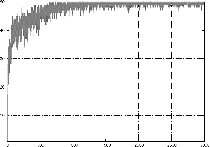
The last functions used to limit the velocity are l and m. They show an unexpected behavior in the experiments. A particular case is SchwefelTwo using function l to limit the velocity. In this case, once the termination criterion of a maximum number of function evaluations is reached, we observed a large number of particles going out of the limits of the search space. As the changes in the limit of the velocity are computed using the number of function evaluations, the limit does not change fast enough. We believe that, since we did not use any other method to reduce the velocity, the particles continued to go out of the limits of the search space, which is the reason why a much larger computational effort is required in this case.
The plot in Figure 6 shows the number of particles that go out of bounds in each cycle. As we can observe, the number of particles out of bounds increases quickly, and close to iteration 1000 almost all the particles are out of bounds of the search space. The method used to handle the particles when they go out of bounds, does not evaluate the particle in its new position. Thus, the best position of the particle is not evaluated either, but the velocity is preserved.
Another method consists on setting the position of the particle to the corresponding limit only in the dimension that is exceeding, i.e., if the particle exceeds the upper limit for the search position in dimension k, then the position of the particle in the kth index is set to Xk,max , or Xk,min as deemed appropriate. The experiments where repeated and the results are shown in Table 4.
Table 4 Comparison of the results of the standard PSO and the li and mi functions
| Function | SPSO | l1 | m1 |
| mean | mean | mean | |
| ackley | 1.9834E+01 | 1.9973E+01 | 2.0000E+01 |
| camelback | 4.6510E-08 | 9.2869E-05 | 5.8087E-08 |
| goldsteinprice | 4.0500E+01 | 7.2902E+01 | 7.8300E+01 |
| griewank | 7.8270E+01 | 1.3388E+02 | 2.1072E+02 |
| penalizedone | 8.5333E+06 | 8.5333E+06 | 1.7067E+07 |
| penalizedtwo | 5.4675E+07 | 9.5681E+07 | 6.8344E+07 |
| rastrigin | 2.6460E+02 | 2.8186E+02 | 4.0506E+02 |
| rosenbrock | 2.6683E+06 | 1.8659E+07 | 3.1972E+07 |
| schwefelone | 4.2088E+04 | 5.6748E+04 | 1.1819E+05 |
| schwefeltwo | 1.7122E+04 | 1.6953E+04 | 1.6723E+04 |
| shekelfive | 5.0524E+00 | 5.0631E+00 | 5.0524E+00 |
| shekelseven | 5.2741E+00 | 5.2850E+00 | 5.2741E+00 |
| shelelten | 5.3608E+00 | 5.3726E+00 | 5.3608E+00 |
| sphere | 1.1000E+04 | 1.5104E+04 | 2.9333E+04 |
We can observe from Table 4 that using the l1 and m1 functions does not produce better results, but the use of the method to limit the position of a particle also affects the results of the SPSO. To achieve better results, it is necessary to find a different method to limit the position of a particle. This will be part of our future research given that the methods to limit the position of a particle require a comprehensive review.
4.4 Learning Constants
The learning constants are adjusted in the SPSO algorithm as well as w in the Inertia Weight model, and x in the Constriction Factor model. In our case, we do not use any factor to limit the velocity. We only use a change in the velocity limit. The results shown in Tables 1, 2, and 3 were computed using the values c1 = c2 = 1.49445. We performed experiments using values of c1 = c2 = 1.0, adopting the h2 and h3 functions, which were the functions that produced the best results to limit the velocity.
From Tables 5 and 6 we can observe that in some cases we have better results but not in all of them. It is worth mentioning that in all cases the results are not too different. By setting the values of the learning constant to c1 = c2 = 1.0, we can obtain good results and we can further simplify the equation to compute the velocity of a particle, which can be written as follows:
Table 5 Comparison of the results of the standard PSO, using the h2 function, and the h2 function with c1 = 1 and c2 = 1.
| Function | SPSO | h2 | h2 |
| c1 = c2 = 1 | |||
| mean | mean | mean | |
| ackley | 1.9733E+01 | 1.2198E-03 | 3.8233E-01 |
| camelback | 4.6510E-08 | 4.6510E-08 | 4.6510E-08 |
| goldsteinprice | 2.4300E+01 | 5.6184E-13 | 1.9394E-12 |
| griewank | 1.7208E-02 | 8.1718E-03 | 1.0389E-02 |
| penalizedone | 1.2097E-01 | 5.3250E-02 | 4.5596E-02 |
| penalizedtwo | 4.6242E-02 | 2.1687E-03 | 2.2044E-03 |
| rastrigin | 1.7113E+02 | 4.6929E+01 | 4.3820E+01 |
| rosenbrock | 4.4084E+01 | 1.1411E+02 | 2.1497E+02 |
| schwefelone | 1.8303E+01 | 1.8257E+00 | 2.1560E+00 |
| schwefeltwo | 1.6349E+04 | 1.7729E+04 | 1.7608E+04 |
| shekelfive | 5.0524E+00 | 5.0524E+00 | 5.0524E+00 |
| shekelseven | 5.2741E+00 | 5.2741E+00 | 5.2741E+00 |
| shelelten | 5.3608E+00 | 5.3608E+00 | 5.0034E+00 |
| sphere | 2.0311E-18 | 3.0900E-05 | 1.1508E-04 |
Table 6 Comparison of the results of the standard PSO, using the h3 function, and the h3 function with c1 = 1 and c2 = 1.
| Function | SPSO | h2 | h2 |
| c1 = c2 = 1 | |||
| mean | mean | mean | |
| ackley | 1.9733E+01 | 3.1058E-02 | 1.9835E-01 |
| camelback | 4.6510E-08 | 4.6510E-08 | 4.6510E-08 |
| goldsteinprice | 2.4300E+01 | 3.6306E-17 | 3.0134E-17 |
| griewank | 1.7208E-02 | 1.1079E-02 | 9.6877E-03 |
| penalizedone | 1.2097E-01 | 1.3823E-02 | 1.0387E-01 |
| penalizedtwo | 4.6242E-02 | 3.6625E-04 | 1.4650E-03 |
| rastrigin | 1.7113E+02 | 4.8521E+01 | 5.5353E+01 |
| rosenbrock | 4.4084E+01 | 1.2790E+02 | 3.3805E+02 |
| schwefelone | 1.8303E+01 | 5.7513E-02 | 1.0583E-01 |
| schwefeltwo | 1.6349E+04 | 1.7673E+04 | 1.7556E+04 |
| shekelfive | 5.0524E+00 | 5.0524E+00 | 5.0524E+00 |
| shekelseven | 5.2741E+00 | 5.2741E+00 | 5.2741E+00 |
| shelelten | 5.3608E+00 | 5.1821E+00 | 5.1821E+00 |
| sphere | 2.0311E-18 | 4.0248E-09 | 2.8470E-08 |
Equation (25) still depends on the best position p of the particle and the global best g of the swarm, but it is simpler.
5 Conclusions and Future Work
We have shown a method to limit the velocity of the particles in the PSO algorithm that was able to produce competitive or even better results than other schemes to limit the velocity of a particle. The proposed approach does not require any factor to limit the velocity of a particle, since it only limits the maximum velocity. This leaves the equation to compute the velocity as simple as the original PSO algorithm. The functions used to limit the maximum value of the velocity are also simple: single term polynomials.
The proposed method can use values for the learning constants equal to one. This selection of values does not affect the performance of the PSO algorithm and, in some cases, it leads to better results. This makes the equation to compute the velocity of a particle even simpler. We concluded with a simple and efficient PSO variant.
Although the values of the learning constants are not critical for the results of the PSO reported in this paper, there are others factors that can affect the performance of the algorithm. The method to limit the position of the particles can be relevant in the overall performance, not only in the final results but in the runtime of the algorithm.
The results of the experiments reported in Tables 1 suggested that more exploration was needed. This hypothesis was rejected by the results in Table 2, where more exploration was performed and the results got worse. The results in Table 2, produced using functions that limited the exploration and favor the exploitation turned out to be better. In future work we will explore different function shapes to find a balance between exploration and exploitation in traversing and searching the feasible search space.
Although the PSO algorithm is well known for its simplicity and its fast execution, there are several factors that can affect its performance. Some of them have already been examined but others have not, e.g., how to limit the position of a particle. It is necessary to examine in detail the implementation of SPSO in all of its phases and determine how the different methods affect its performance.

