


 nueva página del texto (beta)
 Inglés (pdf)
 Artículo en XML
 Referencias del artículo
 Enviar artículo por email
 Citado por SciELO
  Similares en
SciELO
Similares en
SciELO 
 Permalink
1 Introduction
Over the last fifteen years, a popular trend in computer vision (CV) has been the extensive use of locally salient regions to develop solutions for a large variety of visual tasks, such as object detection and recognition, image indexing and retrieval, image stitching, and visual simultaneous mapping and localization. Locally salient regions can be used to uniquely represent an observed scene and construct visual appearance models 22, 33.
1.1 Background
To characterize a particular scene or object through locally salient regions, a general three stage process takes place. First, features need to be detected, using interest point or interest region detectors 33. Second, a unique and informative numerical vector is constructed taking the local image region as input; these vectors are commonly referred to as local image descriptors 22. Finally, the detected image regions and their corresponding local descriptors are used as input to construct a problem specific representation or model. Afterwards, the stored models can be used to detect previously seen features by matching stored visual models with features detected online by the system.
In the process described above, the quality and synergy of a particular detector/descriptor combination is paramount, however the variety of available methods makes it difficult to determine which combination of methods are best suited for common tasks. CV literature is filled with many different proposals, such as the Harris detector 9, Shi-Tomasidetector 27 or the FAST detector 26. In the case of local descriptors, popular algorithms include SIFT 21 and SURF 1, techniques that are now widely used and available in popular programming libraries, such as OpenCV or Matlab toolboxes.
1.2 Experimental Approach
The current paper compares these popular techniques with two more recent approaches towards the feature detection and description problem. In particular, we consider the Harris and Shi-Tomasidetectors and the SURF local region descriptor as standard machine baseline methods. Moreover, we explore other recent approaches to address these tasks.
First, we consider proposals that derive feature extraction algorithms using an automated design process based on meta-heuristic and global search algorithms. In particular, proposals that relied on genetic programming (GP), a form of evolutionary computation 19, to automatically synthesize feature detectors 31, 24, 25 and descriptors 32, 30. In the case of feature detectors, 31, 24, 25 used widely accepted performance measures to pose an optimization problem and solve it using GP to produce novel image operators. Similarly, 30 used GP to optimize the Holder image descriptor 32, providing a fast and simplified feature description algorithm. It is important to note that automatically designing computer vision algorithms through GP is not a commonly used approach within the CV community. Moreover, those works present a limited and controlled experimental validation of the new methods, so it is still not clear if the GP-generated methods can compete with standard techniques in real-world scenarios.
Second, this work proposes a new approach towards feature description, based on popular techniques from statistical image processing and optics literature 8. In particular, we develop a new local description method based on an improved version of the synthetic discriminant filter (SDF) 7, a type of composite correlation filter that is widely used in distortion tolerant object recognition and target tracking applications 14, 12, but not often used in computer vision applications based on local features.
To compare these different paradigms we have chosen a difficult real-world problem, widely addressed in vision based robot navigation, referred to as visual simultaneous localization and mapping, or visual SLAM.
Klippenstein and Zhang 18, 17 also present a comparison of feature extraction methods applied to visual SLAM, using several well-known computer vision methods. The authors used two comparative metrics to evaluate a SLAM system based on the Extended Kalman Filter. First they determine if the estimated trajectory is consistent with the ground truth trajectory, based on the normalized estimation error squared (NEES). However, their results showed that the SLAM system was almost never consistent, so they relaxed this criteria in their comparative work. Therefore, as a second evaluation measure they used the accumulated uncertainty as their comparative measure. Their experimental work showed no significant difference between the considered methods. On the other hand, the recently proposed SLAMBench evaluation platform 23 identifies the average trajectory error (ATE) error as the most important comparative measure between SLAM systems; i.e., the error between the estimated robot trajectory and the ground truth trajectory, This measure is useful since most visual SLAM systems will not produce consistent trajectories, making uncertainty a misleading measure 18,17. Moreover, it is easier to determine the ground truth position and trajectory of the robot than the position of the scene landmarks. However, a more direct comparison of local feature extractors is to consider the accuracy they provide when detecting previously stored landmarks; the main task they are intended to solve. It is also important to consider the computational efficiency of each method, since real-time performance is necessary.
In this work we use the well known Mono-SLAM system of Davison et al. 4, a visual SLAM system that builds a sparse map using local features as landmarks. In all our experimental test, three detectors are considered: two common computer vision approaches (Harris and Shi-Tomasi) and an automatically generated detector (MOP). Also, four local descriptors are tested: Normalized Cross Correlation (NCC, the method used in Mono-SLAM), a common computer vision method (SURF), a GP optimized descriptor (Holder descriptor) and the newly proposed Sdf descriptor. Every detector/descriptor combination is tested on the Mono-SLAM system, using two experimental environments: (1) two paths in a controlled environment where the real trajectory of the robot is known; (2) a freely captured video sequence provided with the Mono-SLAM system.
To evaluate each feature detector and descriptor algorithm, three performance measures are used. Firstly, the average error between the estimated robot trajectory and the ground truth trajectory (ATE), in some experiments a precise ground truth is obtained by using a high-precision industrial robotic arm to perform the trajectory in a hand-eye configuration of the visual SLAM system.
Secondly, an evaluation based on the ability of the system to detect and match previously seen landmarks within the scene, this measure is particularly useful since it only considers the feature matching process.
Thirdly, the computational efficiency of each detector and descriptor algorithm, which is reported in CPU time. Results suggest that the non-standard approaches towards local feature extraction can help to improve the accuracy of the matching process, achieve high quality estimations of the trajectory of the camera produced by the Mono-SLAM system, while also substantially reducing the total computational costs.
1.3 Contributions and Organization
Let us summarize the main contributions of the present research work. First, we propose a new local feature descriptor based on the SDF, a technique from optical and signal processing that is not widely known or studied within the computer vision community. Second, we evaluate and compare a GP-based point detector (MOP), a GP-optimized descriptor (Holder descriptor) and the proposed SDF-based descriptor, with common techniques from CV literature on a difficult real-world problem. Finally, our experimental work suggests that these unconventional approaches to the local feature extraction problem compare favorably with widely used CV techniques.
The paper is organized as follows. Section 2 provides a short review of the more popular methods towards local feature extraction in computer vision systems. Section 3 provides alternative approaches for feature extraction, namely: automatic design methods based on the GP 24, 25, 31, 32, 30 and a method based on composite correlation filtering 7. Section 4 provides a brief overview of the SLAM problem and the Mono-SLAM system. Section 5 presents the experimental work and main results. Finally, Section 6 presents our concluding remarks.
2 Local Feature Extraction Methods in Computer Vision
This section provides a short review of standard approaches towards local feature extraction in computer vision systems. Comprehensive surveys on this topic can be found in 22, 33. Here, we briefly describe some of the more popular methods, particularly those used in the experimental work of this paper. However, lets first summarize the different tasks involved in the local feature extraction process:
- First, an interest point detector is applied to the image, to detect salient and interesting regions in an image. Popular techniques include the Harris and the Shi-Tomasi detector.
- Second, a local descriptor is extracted from the detected regions, to characterize the local image content. Popular techniques include the SIFT and SURF descriptors.
- Finally, these local features are used to characterize image content and solved a higher-level task, such as object recognition or SLAM.
2.1 Interest Point Detectors
Interest points are simple point features within an image; that is, they are image pixels that are salient or unique when compared with neighboring pixels. The algorithms used to detect interest points analyze the intensity patterns within local image regions and only make weak assumptions regarding the underlying structure. Interest points are quantitatively and qualitatively different from other points, and they usually represent only a small fraction of the total number of image pixels.
A measure of how salient or interesting each pixel is can be obtained using a mapping of the form K(x): ℝ+ → ℝ called an interest point operator. Applying the mapping K to an image I produces what can be called an interest image I*. Afterwards, most detectors follow the same basic process: non-maxima suppression that eliminates pixels that are not local maxima, and a thresholding step that obtains the final set of points. Therefore, a pixel x is tagged as an interest point if the following conditions hold,
where W is a square neighborhood of size n x n around x, and h is an empirically defined threshold. The first condition in Equation 1 accounts for non-maximum suppression and the second is the thresholding step (see Figure 1).

Fig. 1 Example of the interest point detection process, where OMOP (I) is the MOP operator and the N(·) represents the non-maxima suppression and thresholding function
The problem of detecting interest points has been well-studied and a large variety of proposals exist in current literature. For instance, the most widely used methods employ image operators that are based on the local second-moment matrix A(x, σI, σD), defined as
where σD and σI are the differentiation and integration scales respectively, Gσ is a Gaussian smoothing function, and Lu = Lu(x, σD) is the Gaussian derivative in direction u of image I at point x. For instance, the interest point operator used by the Harris detector 10 is
where k is a scale parameter, Det defines the determinant and Tr defines the trace. The Shi-Tomasioperator 28 is given by
where λ1; λ2 are the two eigenvalues of A. The subindex of KH and KS-T are used as shorthand to refer to the namesake of each operator.
2.2 Local Image Descriptors
The problem of local image description has been extensively studied and many algorithms have been proposed. One of the most popular local descriptors is the Scale Invariant Feature Transform (SIFT) 21, which is still widely used and available in many computer vision libraries. Similar to other state-of-the-art descriptors, SIFT uses a distribution-based approach, characterizing image information using histograms that attempt to capture the main properties of local shape or appearance. For instance, the simplest approach would be to use histograms of pixel intensities. However, SIFT builds an histogram of the gradient distributions within the detected local region, a 3D histogram of gradient orientations at different locations (discretized by a uniform grid), weighted by the gradient magnitudes. Moreover, random noise is suppressed using bilinear interpolation and a Gaussian function is used to increase the relative importance of pixels near the center of the local region.
One important drawback of the SIFT descriptor is its computational complexity, making it difficult to use in low performance computer systems or in scenarios where real-time response is critical. This is the case of a low cost embedded computing system for a mobile robot that needs to solve a visual SLAM problem.
The Speeded-Up Robust Features (SURF) descriptor was proposed as a more efficient method 1, and it has achieved strong results in many scenarios 3, 11. This descriptor is also distribution-based, building a histogram of Haar-wavelet responses within the interest point neighborhood. Basically, building the SURF descriptor consists of the following steps. First, the dominant gradient orientation of the local image region is determined. Afterwards, a square region is aligned with the dominant orientation. The region is then divided into a 4 by 4 grid, and the Haar-wavelets responses are then estimated based on a uniform sampling, using the sum of the response in each direction (vertical and horizontal) and the sum of the absolute values. Note that a total of four attributes for each subregion are obtained. This gives a descriptor of 64 dimensions, half the size of the SIFT descriptor. Moreover, integral images are used to increase efficiency, since they allow for a fast implementation of box convolution filters.
3 Alternative Approaches for Feature Extraction
In this section, we review alternative approaches towards local feature extraction, based on an automatic design methodology with GP and on image processing techniques with composite correlation filters.
3.1 Automatic Design of Local Feature Extractors with Genetic Programming
It is instructive to consider that most published feature detectors and descriptors are normally accompanied with experimental evidence from a particular domain that illustrates the superiority of the method under some conditions when compared with other techniques. However, such results can rarely provide assurance that a particular method will be well suited for a new or unique scenario. Therefore, researchers have performed extensive experimental evaluations and comparisons of these methods, using domain independent criteria that capture the underlying characteristics that such methods are expected to have 22, 32, 30.
Based on those works, recent contributions have followed the opposite approach, using these experimental criteria as the basis for objective functions, and then posed a search and optimization problem to automatically synthesize high-performance feature detectors or descriptors 24, 25, 31, 32, 30. The general goal is to exploit meta-heuristic and hyper-heuristic search methods to help researchers during the design process of specialized operators. However, we do not suggest that such an approach is in some way superior to a traditional design process. Instead, we agree with 24, hyper-heuristic searchers such as GP can produce novel designs that can assist in the development of high-performance and possibly unconventional solutions to difficult problems. In particular, this paper studies the interest point detector generated with a multi-objective GP 24, 31, 25, and the GP-optimized Holder descriptor from 32, 30, both of which are described next. But first a brief introduction to GP is provided, which is the core algorithm used to derive both operators.
3.1.1 Genetic Programming
Evolutionary algorithms (EA) are population-based search methods, where candidate solutions are stochastically selected and varied to produce new solutions for a specified problem. This process is carried out iteratively until a predefined termination criterion is met. In general, to apply an EA the following aspects must be defined based on domain knowledge. First, an encoding scheme to represent and manipulate candidate solutions for a given problem. Second, an evaluation or fitness function f that measures the quality of each solution based on the high-level goal of the problem. Third, an EA applies variation operators that take one or more solutions from the population as input and produce one or more solutions as output. Fourth, solutions are chosen by the variation operators based on their fitness using a predefined selection mechanism. Finally, a survival strategy decides which individuals within the population will appear in the following iteration.
Among EAs, GP is arguably the most advanced technique, since it can be used for automatic program induction 20. In standard GP each individual is represented by a syntax-tree, because such structures can efficiently express simple computer programs, functions, or mathematical operators. Tree nodes contain a single element from a specified finite set of primitives P = T ∪ F. Leaf nodes contain elements from the set of terminals T, which normally correspond to inputs, while internal nodes contain elements from the set of functions F, which are the basic operations used to build more complex expressions. In essence, P defines the nature of the underlying search space for the evolutionary search, and even when a maximum depth or size limit for individual trees is enforced, normally the search space is very large but finite.
3.1.2 Multi-Objective Interest Point Detector
In 24, 25, a multi-objective GP was used to design the MOP point detector, optimized based on two competing objectives, point dispersion and repeatability rate. The terminal set included the input image, as well as first and second order derivatives, which are widely used by other interest point detectors. The function set included several arithmetic operations and image filters, also based on the type of operations performed by a large subset of point detectors. The multi-objective search was carried out using the second version of the Strength Pareto Evolutionary Algorithm (SPEA-2) 34 and implemented using the GPLAB Matlab toolbox for GP 29.
The final MOP detector was constructed by carefully analyzing the Pareto front and the Pareto-optimal set of solutions generated by the GP search. The symbolic expression of the MOP operator OMOP is
where I is the input image, Gσ denotes Gaussian smoothing filters with scale σ, h = 0.05 is a weight factor that controls the disparity of the detected points, and * denotes convolution operation. After applying the MOP operator, non-maxima suppression and thresholding are used to select the interest points; this process is illustrated in Figure 1. The experimental work presented in 24, 25 clearly showed that the MOP detector performed quite competitively, in terms of repeatability and robustness using standard benchmarks.
3.2 GP-Optimized Regularity-based Descriptor
The Holder descriptor was proposed in 32, and is based on capturing the regularity (or irregularity) of each element of a 2D signal, given by the pointwise Holder exponent. After computing the regularity of each image element, we are left with a regularity matrix H, that characterizes how the signal varies over the image plane. Then, for an image region extracted with an interest point detector, the Holder descriptor is constructed by sampling the regularity matrix in a polar grid around the central point, and ordering the sampling based on the dominant orientation; this process is illustrated in Figure 2.

However, as noted in 32, the Holder descriptor is not useful in real-time scenarios given the high computational cost of estimating the Holder exponent for each image point. Therefore, in 30 GP is used to synthesize an operator OHolder to estimate image regularity more efficiently, given by
The proposed evolutionary process used a similar function and terminal set as the one proposed in 24, 25, and was also implemented in GPLAB 29. Two different fitness functions were used to drive the search process. First, the goal was to evolve operators that could compute the ground-truth regularity of synthetically generated images, where the underlying regularity can be prescribed and is given as the ground truth. While the evolved operators achieved a high accuracy on the synthetic images, they were overfitted and did not generalize to real-world scenes.
Therefore, the second approach was to reproduce the estimated regularity of a known but computationally expensive method. In 30 we showed that the operator generated by GP could estimate image regularity at a fraction of the computational cost of traditional methods, without sacrificing performance on the feature description problem evaluated over a set of standard benchmarks. However, such as in 24, 25, the evolved operators have not been evaluated in real-world scenarios, where the computed local features are used as input to a higher level process. In what follows, the SLAM problem is described emphasizing how local image features are used in this common robotics task.
3.3 Synthetic Discriminant Functions Filter for Local Feature Description
Composite correlation filters are widely used for distortion tolerant object recognition, and in tracking applications for computer vision 16, 2. These filters represent the impulse response of a linear system designed in such a manner that the coordinates of the system's maximum output are estimates of the target's location within an observed scene. In the last decades plenty of proposals have been suggested for the design of composite filters for distortion tolerant pattern recognition, by optimization of several performance criteria 16.
In the present work, we are interested in the design of a filter capable of matching a local image feature when it is embedded in a disjoint background and the observed scene is corrupted with additive noise. Additionally, the filter must be able to recognize geometrically distorted versions of the target, such as rotated and scaled versions.
Let I = {ti(x,y); i = 1, ⋯, N} be a set of availabe image templates representing different views of the image feature t(x, y) to match. We assume that the observed scence patch f(x, y) contains an arbitrary view of the target ti (x, y) embedded into a disjoint background b(x, y) at unknown coordinates (τx, τy), and the image is corrupted with zero-mean additive white noise n(x, y), as follows:
where
In Equation 7, T(u, υ) and
To successfully employ the MF for the feature description problem used by a SLAM system, the following issues must be addressed. First, the support function
Note that the target can be located at any coordinates within the observed scene patch. Thus the support function of the whole patch can be taken as
Now, suppose that the background within the scene patch has a separable exponential covariance function; then, Pb(u, υ) can be computed as 13
where
Furthermore, assume that the noise-free image
Now, let hi(x, y) be the impulse response of a MF constructed to match the ith available view of the target ti(x, y) in I. Let H = {hi(x, y); i = 1, · · · , N} be the set of all MF impulse responses constructed for all training images ti(x, y). We want to synthesize a filter capable to recognize all target views in I, by combining the optimal filter templates contained in H, and by using only a single correlation operation. The required filter p(x, y) is designed according to the SDF filter model, whose impulse response is given by 16
where {αi; i = 1,⋯, N} are weighting coefficients that are chosen to satisfy the following conditions: 〈p(x, y), ti(x, y)〉 = ui; where "<, >" denotes inner-product, and u are prespecified output correlation values at the origin, produced by the filter p(x, y) in response to the training patterns ti(x, y).
Let us denote a matrix R with N columns and d rows (d is the number of pixels), where its ith column contains the elements of the ith member of H in lexicographical order. Let a = [αi; i = 1,⋯,N]T be a vector of weighting coefficients. Thus, Equation 11 can be rewritten as
Furthermore, let u = [ui = 1; i = 1..., N]T be a vector of correlation constraints imposed to the filter's output in response to the training patterns ti(x, y), and let Q be a d x N matrix whose ith column is given by the vector version of the ith view of the target in I. Note that the filter's constraints can be expressed as
where superscript "+" denotes conjugate transpose. By substituting (12) into (13), we obtain u = Q+ Ra. Thus, if matrix Q+ R is nonsingular the solution for a, is
Finally, by substitution of (14) into (12), the solution for the SDF filter is given by
For the purpose of local feature description, we propose the following process based on the SDF filter design, depicted in Fig. 3. First, given an interest point x, we extract a scene patch of 11 x 11 pixels around x; this represents our reference target pattern t(x, y). Next we create two synthetically rotated versions of t(x, y), one rotated 15 degrees clockwise and another rotated 15 counterclockwise, and construct a three element set I. Next, set H is created by syhthetising the MF impulse responses of all patterns in I. Finally, an SDF filter template is synthesized with Equation 15.

4 Visual-based Simultaneous Localization and Map Building
When a robot is placed in an unfamiliar place an important task is to gradually build a map of the surrounding environment and simultaneously determine the current location within this map. This is formally known as the SLAM problem 6. One approach towards solving SLAM is through computer vision techniques, where a camera is used as the navigation sensor and CV techniques are used to extract and analyze the captured information (for instance, detection and description of locally salient features). An example of this approach is the Mono-SLAM system developed by Davison et al. 4. Mono-SLAM is a real-time algorithm that solves the problem of SLAM using a monocular camera as its only sensor, from which it recovers a 3D trajectory and map of its environment.
Mono-SLAM has to overcome several challenges, starting with the fact that it cannot determine the depth of an object with just one frame capture of the scene. Instead, it requires several views of the same scene, and it must account for the fact that the pose of the camera can change during operation. Other challenges are the unconstrained movement of the camera, and being able to perform real-time localization. With this in mind, Mono-SLAM solves these, and other challenges, using a specialized initialization procedure. This procedure combines several techniques such as the extended Kalman filter (EKF), a particle filter, an active search heuristic, as well as local feature detection and matching to identify and recognize useful landmarks. We begin our overview of Mono-SLAM with the initialization step. First, the intrinsic parameters of the camera must be obtained off-line through calibration. Afterwards the extrinsic pose parameters of the camera (robot) are determined relative to a fixed initialization pattern. This process is needed to initialize the state vector in the prediction step of the EKF. Next, the operation of the EKF encompass three basic steps, prediction, measurement and correction. First, the state vector X and covariance matrix P of the system are given by,
where
rW is a 3D position vector, qWR is the orientation quaternion, υW is the velocity vector, and wR is the angular velocity vector relative to a fixed world frame W and camera frame R. After initialization, the first step is prediction, which provides prior knowledge of where the next position of the camera and features might be. In this stage, the algorithm runs a visibility test to determine if the known features are visible; those that do not pass this test remain as unused features, otherwise they are marked for measuring and those with the highest level of uncertainty (large covariance) are selected. Second, the measuring step is divided into two tasks, active search and matching. The active search is a method that reduces the amount of computational cost of searching for a feature within an image, using the camera model and knowledge of the predicted localization of previously detected features. In this case we are searching for a given feature within a local neighborhood given by the predicted location and the associated uncertainty. Afterwards, features are matched within the predicted search region of the image, if the match is true then the feature is labeled as a match and it is labeled as a non-match otherwise. If a feature cannot be successfully matched after a certain number of attempts, the feature is discarded. Third, the correction step is performed on the state vector to reduce the uncertainty of the location of the camera and each feature. After the EKF, map maintenance continues by performing a detection of new landmarks and using a particle filter to obtain an initial position estimate. To detect new features, an interest point detector is applied within a search box using a heuristic rule, to search for new features when the map is too sparse, and only doing so in scene regions that do not already contain other visible landmarks, by considering the movement model and avoiding image boundaries. The particle filter is used to determine the depth of a newly detected feature; that is, there is no knowledge of the depth of the feature when it is first detected and the particle filter estimates it by tracing a line from the first view of the feature and the current pose of the camera, and filling the line with a uniformly distributed set of candidate 3D locations. Then, in an iterative process it attempts to match the particles until they form a Gaussian distribution, at which point the features are fully initialized and marked as unused. This sequence of steps if performed in a loop, as depicted in Figure 4.

Fig. 4 Block diagram of the main processes within Mono-SLAM, the blocks for local feature detection and description (the darker solid block and dotted block respectively) are emphasized
It is important to note that the Mono-SLAM system depends on the quality of two low-level processes, feature detection and description, in order to add and recognize landmarks within the 3D map. The original Mono-SLAM system utilizes the Shi-Tomasi detector in combination with basic normalized cross-correlation for feature matching.
5 Experiments and Results
As stated before, the goal of the experimental work is to evaluate the performance of a particular detector/descriptor combination when it is used within a visual SLAM system; all of the combinations tested in this work are summarized in Table 1. These methods are evaluated using the Mono-SLAM system implemented in SceneLib2 by Hanme Kim1, which is an extension of Davison's original SceneLib1. The camera used in the experiments is a low-cost IEEE 1394 web-cam with a frame rate of 30fps and an image resolution of 320 x 240 pixels. The camera calibration parameters are: the horizontal and vertical focal lengths are fku = fkυ = 195 pixels, the principal point is (u0, υ0) = (162,125), and the distortion coefficient is K1 = 6 x 1076. The Mono-SLAM system is executed on a PC running on Ubuntu Linux 12.04 LTS operating system with an Intel® Xeon(R) CPU E3-1226 v3 @ 3.30GHz with 4 cores. The MOP and Harris detectors, as well as the Holder, SDF and SURF descriptors were implemented in C++ using the OpenCV v2.4.2 library. The MOP detector, Holder descriptor and SDF filters are available in the GPCV (GP for computer vision) library under de GPL license, available at www.tree-lab.org/index.php/gpcv.
Table 1 Summary of the detector/descriptor combinations used in this work
| Detector | Descriptor |
| Shi-Tomasi | NCC |
| Shi-Tomasi | SURF |
| Shi-Tomasi | Holder |
| Shi-Tomasi | SDF |
| MOP | NCC |
| MOP | SURF |
| MOP | Holder |
| MOP | SDF |
| Harris | NCC |
| Harris | SURF |
| Harris | Holder |
| Harris | SDF |
The presented experimental work evaluates the following performance measures:
- The number of scene features (landmarks) that are correctly Matched at each iteration of the Mono-SLAM system.
- The ATE (average trajectory error), computed using the root mean squared error (RMSE) between the estimated trajectory and the ground truth.
- The eficiency of each feature detector and descriptor, based on the required CPU time.
The work considers two test scenarios. In the irst scenario the ground truth trajectory is known, generated by a camera mounted on the end effector of a Staubli RX-60 manipulator robot with six degrees of freedom in a hand-eye coniguration, as shown in Figure 5. Two test trajectories are generated, respectively referred to as Experiment A and Experiment B.

Fig. 5 Physical scenario of the robot RX-60 with a webcam mounted in its end efectorto generate the reference trajectories
Experiment A uses a sine trajectory, where the camera moves 0.14 meters across the z axis (amplitude of the sine) and 0.5 meters along the x axis, with no change in image scale (y axis of the robot frame of reference). Experiment B uses a straight line trajectory, where the camera moves 0.3 meters in all axes. In both experiments, the image plane of the camera is parallel to the x - z plane of the robot's coordinate system, with y representing a change in scale. The ground truth trajectory of each experiment is presented in Figure 6. As shown in Figure 5, the experiments are carried out in an ofice environment with posters and paintings on the walls to provide texture and interesting visual features. The ground truth trajectory is known with a precision of 0.05 millimeters according to the Staubli RX-60 speciication. The video captured by the camera is recorded for offline processing by the the Mono-SLAM system; however the system can operate online at 30fps.

The second test scenario presents a less controlled environment, referred to as Experiment C. For this experiment, the video sequence is provided with SceneLib2, which has an image resolution of 320 x 240 pixels and the Mono-SLAM system requires 500 iterations to process the entire video sequence; four sample frames of this test video are shown in Figure 7. The Mono-SLAM system is executed 30 times using the test video from each experiment (A-C), to account for the stochastic processes used by Mono-SLAM. Finally, rank statistics over all runs are used to compare each detector/descriptor combination.

5.1 Experimental Setup
The Mono-SLAM system is conigured to use 10 visible features at each iteration with a patch size of 11 x 11 pixels. The parameters of the methods are given in Table 2.
Table 2 Parameters used with each method
| Method | Parameter |
| Shi-Tomasi | Default values of Scenelib library |
| Harris | k = 0.04 |
| Non-Maxima Suppression: Block size = 10 pixels; Threshold = 0.9 | |
| MOP | h = 0.5; |
| Non-Maxima Suppression: Block size = 5 pixels; Threshold = 0.9 | |
| NCC | Default values of Scenelib library |
| SURF | Descriptor vector size = 64 |
| Hölder | Descriptor vetor size = 64 |
| SDF | Γ = 0.005, ρx = ρy = 0.80 |
The parameters in Table 2 were experimentally tuned to obtain the lowest ATE for each detector/descriptor combination. To determine a match for the SURF and Holder descriptors the Euclidean distance between two descriptors is computed, and a match is scored if the distance is below a threshold tm. Similarly for the SDF and NCC descriptors, a threshold for the output correlation peak tc is used to determine a positive match. The values of the threshold vary for each descriptor to obtain the best possible performance; the threshold values are given in Table 3.
5.2 Results
As stated above, the experimental results are presented based on performing 30 independent runs of the Mono-SLAM system with each detector/descriptor combination for each experiment. For experiments A and B, where the ground truth is known, a graphical representation is provided by plotting the average estimated trajectories relative to the ground truth. We group the results based on the interest point detector used and we show the trajectories from four different perspectives: a 3D view, and a view from each plane from the robot's frame of reference (X-Z, Z-Y, X-Z). Additionally, the median of the ATE and of the total correct matches are provided for each detector/descriptor combination. For the number of correct matches, we first take the median number of matches over all the iterations of the system, and then take the median over all 30 runs. In the best case scenario, the trajectory error should be close to zero, while the number of total matches should tend to the total number of visible features (10 in our setup). Statistical tests are performed using a 1XN setup (N methods are compared with a single control method), where the base Mono-SLAM detector/descriptor combination (Shi-Tomasi/NCC) is used as the control method against which all other methods are compared. The non-parametric Friedman test is used to perform the statistical tests, and the resulting p-values are corrected by the Bonferroni-Dunn method. The null hypothesis is rejected at the α = 0.05 confidence level.
Finally, to test the efficiency of each method the following procedure is performed. We use a single highly textured image of 640x480 pixels. Then we detect a total of 100 interest points and extract 100 corresponding feature vectors. The total CPU time required to detect and describe these interest points is also reported.
5.2.1 Experiment A
Figures 8 to 10 show the average estimated trajectories of each detector/descriptor combination for Experiment A. For the Harris detector (Figure 8), the SDF descriptor provides the best trajectory estimation. For the MOP detector (Figure 9), SDF also provides a good estimation, as well as the Hölder descriptor, while the SURF descriptor is noticeably worse. Finally, for the Shi-Tomasi detector, the best estimation is achieved by the Hölder descriptor, while NCC and SURF are noticeably worse.

Fig. 8 Illustrations of the average estimated trajectories for the Harris detector for experiment A; where (a) 3D view, (b) X-Y plane view, (c) Y-Z plane view, (d) X-Z plane view

Fig. 9 Illustrations of the average estimated trajectories for the MOP detector for experiment A; where (a) 3D view, (b) X-Y plane view, (c) Y-Z plane view, (d) X-Z plane view
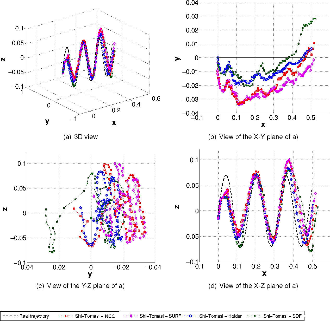
Fig. 10 Illustrations of the average estimated trajectories for the Shi-Tomasi detector for experiment A; where (a) 3D view, (b) X-Y plane view, (c) Y-Z plane view, (d) X-Z plane view
Table 4 summarizes the numerical comparisons for Experiment A and Table 5 provides the p-values of the statistical tests. For this experiment, the ATE of the system appears to be quite robust with respect to the detection/description process, except for two outliers that did exhibit a statistical difference with respect to the control method, these are: ST-SDF and MOP-NCC. While the MOP-Hölder combination shows the best ATE, the only combination that is statistically different with respect to the control method is ST-SDF, while MOP-NCC is the only combination that is statistically worse. However, if we focus on the quality of the detection, description and matching of visual landmarks the results are somewhat different. The median and maximum values are very similar for all combinations, but several methods do outperform the control method, these are: ST-SURF, ST-Hölder, ST-SDF, MOP-SURF, MOP-Hölder, MOP-SDF, Harris-NCC and Harris-Hölder. In summary, for Experiment A the ST-SDF combination is able to improve system performance based on both the ATE and the total correct matches. Similarly, MOP-Hölder also exhibited a noticeable improvement relative to the base Mono-SLAM algorithms.
Table 4 Numerical comparisons for Experiment A, where bold indicates best results
| Experiment A | Match | ATE [meters] | |||
| Max | Median | Max | Min | Median | |
| ST-NCC | 10 | 7 | 0.0551 | 0.0371 | 0.0471 |
| ST-SURF | 10 | 8 | 0.0543 | 0.0353 | 0.0446 |
| ST-Hölder | 10 | 7 | 0.0554 | 0.0343 | 0.0431 |
| ST-SDF | 10 | 6 | 0.0549 | 0.0363 | 0.0466 |
| MOP-NCC | 9 | 6 | 0.0566 | 0.0391 | 0.0502 |
| MOP-SURF | 8 | 5 | 0.0559 | 0.0370 | 0.0469 |
| MOP-Hölder | 10 | 7 | 0.0523 | 0.0335 | 0.0422 |
| MOP-SDF | 10 | 8 | 0.0544 | 0.0365 | 0.0450 |
| Harris-NCC | 10 | 8 | 0.0569 | 0.0354 | 0.0445 |
| Harris-SURF | 10 | 7 | 0.0555 | 0.0358 | 0.0442 |
| Harris-Hölder | 10 | 8 | 0.0546 | 0.0353 | 0.0441 |
| Harris-SDF | 10 | 7 | 0.0554 | 0.0343 | 0.0431 |
Table 5 Results of the 1xN statistical tests, showing the p-values of the Friedman test after Bonferroni-Dunn corrections for Experiment A, with ST-NCC as the control method; bold indicates that the null hypothesis is rejected at the a = 0.05 confidence level
| Experiment A ST-NCC | ST-SURF | ST-HOL | ST-SDF | MOP- NCC | MOP-SURF | MOP-HOL | MOP-SDF | HA- NCC | HA-SURF | HA-HOL | HA-SDF |
| ATE | 1.5854 | 3.0065 | 0.0000 | 0.0001 | 1 1.0000 | 0.1165 | 3.0065 | 5.1173 | 5.1173 | 0.3131 | 3.0065 |
| Match | 0.0071 | 0.0005 | 0.0464 | 1 1.0000 | 0.0046 | 0.0439 | 0.0194 | 0.0469 | 9.2563 | 0.0046 | 2.2091 |
5.3 Experiment B
In this experiment, while the trajectory is simpler than the one used in Experiment A, it introduces scale changes in the observed scene which were not present in Experiment A. This is an important issue, since the interest point detectors (Harris, ST and MOP) are not scale invariant, so the detection process is expected to degrade relative to the performance reported for Experiment A. Therefore, the heavy lifting in the detection process must be done by the feature descriptors extracted from the scene. Moreover, while scale invariant detectors do exist, they are computationally expensive and would degrade system efficiency substantially 33.
Table 6 summarizes the numerical comparisons for Experiment B and Table 7 provides the p-values of the statistical tests. For this experiment, the ATE of the system is more dependent on the detection/description process. We observe much larger performance differences, the median ATE of the best method (MOP-Hölder) is about 70% smaller than the ATE of the worst (ST-NCC). In this case, all combinations are statistically different with respect to the control method, based on the p-values that allow us to reject that null hypothesis. Therefore, to determine the best overall method a multigroup statistical test is performed using an NxN (all pairwise comparisons of N methods) approach with all pairwise comparisons done the Friedman test, and p-values corrected using the Holm procedure. Results are reported in Table 8, where bold indicates that the null hypothesis is rejected at the α = 0.05 confidence level. This table clearly shows that the best ATE performance is achieved by the MOP-Hölder, MOP-NCC and MOP-SURF combinations, suggesting that the MOP detector provides the best detection under scale changes. Figure 11 shows the estimated trajectories obtained with MOP-Hölder, MOP-NCC, MOP-SURF and the control method ST-NCC.
Table 6 Numerical comparisons for Experiment B, where bold indicates best results
| Experiment B | Match | ATE [meters] | |||
| Max | Median | Max | Min | Median | |
| ST-NCC | 10 | 7 | 0.0497 | 0.0315 | 0.0424 |
| ST-SURF | 10 | 9 | 0.0245 | 0.0101 | 0.0187 |
| ST-Hölder | 10 | 9 | 0.0258 | 0.0101 | 0.0173 |
| ST-SDF | 10 | 9 | 0.0257 | 0.0090 | 0.0186 |
| MOP-NCC | 10 | 8 | 0.0222 | 0.0100 | 0.0168 |
| MOP-SURF | 10 | 10 | 0.0234 | 0.0080 | 0.0127 |
| MOP-Hölder | 10 | 10 | 0.0213 | 0.0060 | 0.0126 |
| MOP-SDF | 10 | 9 | 0.0262 | 0.0078 | 0.0181 |
| Harris-NCC | 10 | 7 | 0.0235 | 0.0098 | 0.0159 |
| Harris-SURF | 10 | 9 | 0.0231 | 0.0082 | 0.0137 |
| Harris-Hölder | 10 | 10 | 0.0229 | 0.0078 | 0.0133 |
| Harris-SDF | 10 | 9 | 0.0231 | 0.0090 | 0.0155 |
Table 7 Results of the 1xN statistical tests, showing the p-values of the Friedman test after Bonferroni-Dunn corrections for Experiment B, with ST-NCC as the control method; bold indicates that the null hypothesis is rejected at the α = 0.05 conidence level
| Experiment B | ST-SURF | ST-HOL | ST-SDF | MOP- NCC | MOP-SURF | MOP-HOL | MOP-SDF | HA- NCC | HA-SURF | HA-HOL | HA-SDF |
| ATE | 0.0000 | 0.0000 | 0.0000 | 0.0000 | 0.0000 | 0.0000 | 0.0000 | 0.0000 | 0.0000 | 0.0000 | 0.0000 |
| Match | 0.0000 | 0.0000 | 0.0000 | 0.0120 | 0.0000 | 0.0000 | 0.0000 | 4.0820 | 0.0000 | 0.0000 | 0.0000 |
Table 8 Results of the NxN pairwise statistical tests of the ATE, showing the p-values of the Friedman test after Holm corrections for Experiment B; bold indicates that the null hypothesis is rejected at the α = 0.05 conidence level
| Experiment B | ST- NCC | ST-SURF | ST-HOL | ST-SDF | MOP- NCC | MOP-SURF | MOP-HOL | MOP-SDF | HA- NCC | HA-SURF | HA-HOL | HA-SDF |
| ST- NCC | - | 0.0000 | 0.0000 | 0.0000 | 0.0000 | 0.0000 | 0.0000 | 0.0000 | 0.0000 | 0.0000 | 0.0000 | 0.0000 |
| ST-SURF | - | - | 4.9382 | 4.9382 | 0.0000 | 0.0019 | 0.0005 | 0.0732 | 1.8737 | 0.0078 | 0.0005 | 1.8737 |
| ST-HOL | - | - | - | 4.2900 | 5.1972 | 0.0001 | 0.0000 | 3.5750 | 0.0000 | 0.0000 | 0.0000 | 0.0000 |
| ST-SDF | - | - | - | - | 0.0007 | 0.0030 | 0.0019 | 0.0284 | 1.1541 | 0.0284 | 0.0274 | 1.1541 |
| MOP- NCC | - | - | - | - | - | 0.2998 | 0.0264 | 0.0254 | 2.8600 | 1.0862 | 0.2998 | 2.1450 |
| MOP-SURF | - | - | - | - | - | - | 1.8280 | 0.0244 | 0.0001 | 5.1972 | 1.4300 | 0.0004 |
| MOP-HOL | - | - | - | - | - | - | - | 0.0078 | 0.0000 | 0.0001 | 0.0007 | 0.0000 |
| MOP-SDF | - | -- | - | - | - | - | - | - | 3.0065 | 0.2117 | 0.0351 | 3.0065 |
| HA- NCC | - | - | - | - | - | - | - | - | - | 0.0000 | 0.0000 | 0.0007 |
| HA-SURF | - | - | - | - | - | - | - | - | - | - | 0.0000 | 0.0000 |
| HA-HOL | - | - | - | - | - | - | - | - | - | - | - | 0.0000 |
| HA-SDF | - | - | - | - | - | - | - | - | - | - | - | - |
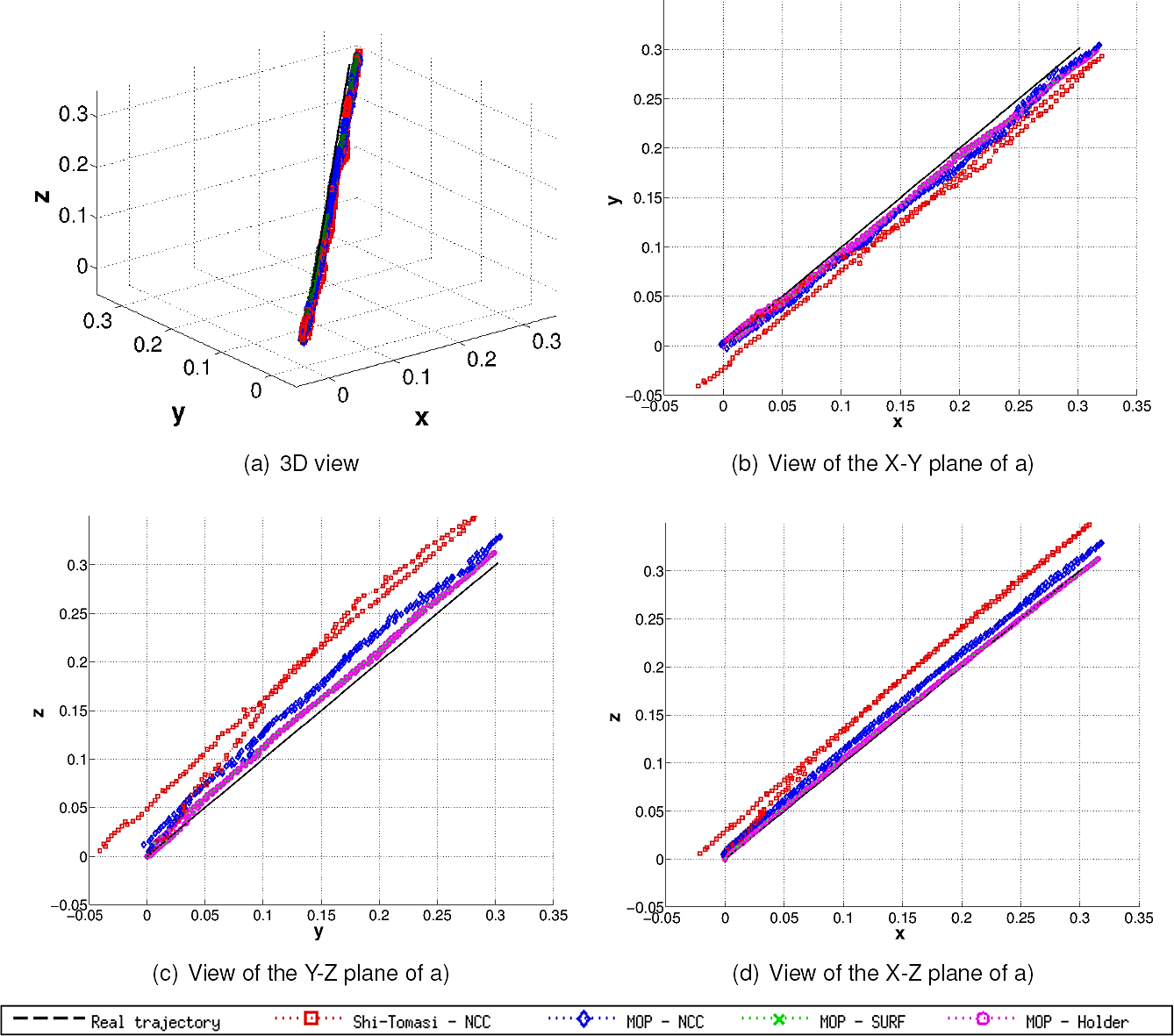
Fig. 11 Illustrations of the estimated trajectories of the best detector/descriptor combinations for Experiment B: (a) 3D view, (b) X-Y plane view, (c) Y-Z plane view, (d) X-Z plane view
In the case of feature matching, results are quite similar. Most detector/descriptor combinations (except Harris-NCC) outperform the control method. In particular, once again the MOP-Hölder and MOP-SURF combinations achieve the best performance, along with Harris-Hölder. This suggest that the Hölder descriptor is robust to scale changes even without the use of a scale invariant detector. For this scenario both of the methods that were automatically designed by a GP search (MOP and Hölder) exhibit the best performance.
5.4 Experiment C
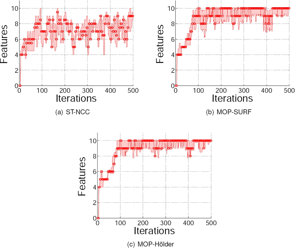
Table 10 summarizes the numerical comparisons for Experiment C and Table 9 provides the p-values produced by the statistical tests. For this experiment, since the ground truth trajectory is not known, we only compare the detector/descriptor combinations based on matching performance. The median values of the total correct matches suggest that most combinations outperform the control method; in particular MOP-SURF and MOP-Hölder exhibit the best performance with perfect median values. Moreover, the statistical tests show that the null hypothesis is rejected in all cases except for the ST-NCC combination. The Shi-Tomasi detector exhibits the worst performance, while the MOP detector achieves the best overall performance. To visualize these results, Figure 12 compares the matching performance of the control method and the best detector/descriptor combinations: MOP-SURF and MOP-Hölder. The plots show the median value of correct matches over all runs of the system at each iteration, plus/minus the irst and third quartiles. Notice that the maximum number of possible correct matches at each iteration is 10, which is achieved at many iterations by the MOP-SURF and MOP-Hölder combinations, but not by ST-NCC. These plots conirm that matching performance in the Mono-SLAM system can be greatly improved by the appropriate detector/descriptor combination.
Table 9 Results of the 1xN statistical tests, showing the p-values of the Friedman test after Bonferroni-Dunn corrections for Experiment C, with ST-NCC as the control method; bold indicates that the null hypothesis is rejected at the α = 0.05 conidence level
| Experiment C | ST-SURF | ST-HOL | ST-SDF | MOP-NCC | MOP-SURF | MOP-HOL | MOP-SDF | HA-NCC | HA-SURF | HA-HOL | HA-SDF |
| Match | 0.0026 | 0.0005 | 4.4592 | 0.0014 | 0.0000 | 0.0000 | 0.0000 | 0.0006 | 0.0000 | 0.0000 | 0.0000 |
Table 10 Numerical comparisons of matching performance in Experiment C, where bold indicates best results
| Experiment C | Match | |
| Max | Median | |
| ST-NCC | 10 | 7 |
| ST-SURF | 10 | 8 |
| ST-Holder | 10 | 8 |
| ST-SDF | 10 | 7 |
| MOP-NCC | 10 | 8 |
| MOP-SURF | 10 | 10 |
| MOP-Holder | 10 | 10 |
| MOP-SDF | 10 | 9 |
| Harris-NCC | 10 | 8 |
| Harris-SURF | 10 | 9 |
| Harris-Holder | 10 | 9 |
| Harris-SDF | 10 | 9 |
5.5 Comparison of CPU Time
Finally, we evaluated each method based on the total CPU time required to either detect a 100 interest points or build their corresponding descriptors; the results are given in Table 11. First, it is clear that all detectors require about the same computational time, with Harris the slightly slower method and MOP the fastest. On the other hand, the differences between the descriptors are larger. While SURF and SDF are relatively similar, though SDF is faster by 3 ms, the Hölder descriptor is one order of magnitude faster than all other methods, requiring about half the time of the popular SURF descriptor. Given the strong performance achieved by Hölder on the tests reported above, this descriptor is recommended for use in future applications.
6 Concluding Remarks
The detection and description of local features is by now one of the most widely used computer vision approaches. This paper evaluates three different paradigms for local feature construction on the dificult real-world problem of vision-based SLAM. In particular, we test the following paradigms: (1) standard computer vision techniques; (2) automatically generated methods with genetic programming; and (3) an alternative paradigm based on synthetic correlation filters, an original proposal of the current paper.
The experimental work is based on Davison's Mono-SLAM system, using several different experimental scenarios and considering the following performance criteria: the average trajectory error between the estimated camera trajectory and a ground truth trajectory; the quality of the matching process given by the total number of correct matches; and the CPU time required by each method.
The reported results are revealing, suggesting that non-traditional techniques, based on automatic feature construction with GP and SDF iltering, outperform the standard vision techniques considered in this work, such as the SURF descriptor and the Shi-Tomasi detector. This is particularly true when the vision system experiments scale changes and when considering the quality of the matching process. Moreover, GP generated detectors and descriptors are more eficient than standard techniques for feature detection and description.
Future work will focus on exploring other application domains for the MOP detector, and the Hölder and SDF descriptors, given their good performance and computational eficiency compared to standard techniques.
Moreover, the automatic generation of feature extraction methods with GP could be carried out online, to ind specialized features for speciic environments in real-time.

