


 nueva página del texto (beta)
 Inglés (pdf)
 Artículo en XML
 Referencias del artículo
 Enviar artículo por email
 Citado por SciELO
  Similares en
SciELO
Similares en
SciELO 
 Permalink
1 Introduction
As part of an experimental process, it is common to face up to situations where only a limited
amount of data is available and the estimation of values between consecutive data
points is needed, either for predicting results or inferring conclusions from data.
Although this problem is traditionally approached by function approximation methods
based on polynomial interpolation, a preferred alternative can be found in the
approximation techniques based on piecewise-linear models 7,
16,
17,
5,
4 which consists in connecting
consecutive data points by straight line segments through a continuous function.
However, piecewise-linear models have the shortcomings of having zero curvature
between data points, exhibiting abrupt changes at the breakpoints, and having
undefined derivatives. It is precisely the lack of differentiability what limits
their application in such cases where, as a result of derivative computations, the
function
The paper is organized as follows. In Section 2, the absolute-value function that serves as kernel for the High Level Canonical piecewise-linear model is presented. Section 3 describes the methodology for constructing smooth-piecewise functions. Section 4 shows the application of such methodology by illustrative examples (for one- and two-dimensional domains). In Section 5 a comparative analysis and discussion about the curve fitting accuracy that can be achieved through the proposed strategy is exposed. The comparison is done among polynomial, splines, smooth-piecewise, and standard piecewise-linear approximation techniques. Finally, Section 6 presents the concluding remarks of this work.
2 Absolute-value Basis-function
A relationship between piecewise-linear models and the absolute-value function is established and reported in many references. Mathematical expressions such as the canonical form of Chua-Kang 3, 15, 1, 2, the High Level Canonical representation of Pedro-Julian et al. 11, 8, the Guzelis 6 model, and the Kahlert 13, 14 description are emblematic examples where this function appears implicitly. Specifically, in the High Level Canonical model the basis-function (also expressed in terms of absolute-value functions) is outlined and easily identified in a detailed methodology by which the approximation function can be constructed. Moreover, this construction methodology is widely reported in literature 10, 9. For these reasons, the smoothing technique which is proposed in this paper takes as reference the basis-function γ(fi , fj) used in the Pedro-Julian et al. 8 model.
where fi and fj are linear equations used to sketch the linear partitions of the function domain.
3 Methodology for the Construction of Smooth-Piecewise Functions
Based on the methodology of Pedro-Julian et al. 8, our proposal for the construction of smooth-piecewise functions can be summarized as follows.
1. Consider as input the set D of N-data that contains the breakpoints coordinates of an arbitrary piecewise-linear function. For the one-dimensional case
D = {(X1, Y1), (X2, Y2), …, (Xi, Yi)}, while for the two-dimensional case
D = {(X1, Y1, Z1), (X2, Y2, Z2),·…, (Xi, Yi , Zi)} with i = 1,2,···,N..
2. Define the basis-function γ(fi , fj). In this step, a suitable approximation for the absolute-value function is used. In accordance with reference 18 a smooth approximation to absolute-value function is given by
where the plus function (x)+ can be approximated by
After combining equation (3) with equation (2), the following smooth approximation is obtained:
After numerical simulations on equation (4), a slight deviation from the absolute-value function can be observed. In order to obtain more accurate fitting, a constant β is included as
However, taking into account the logarithmic change-of-base formula
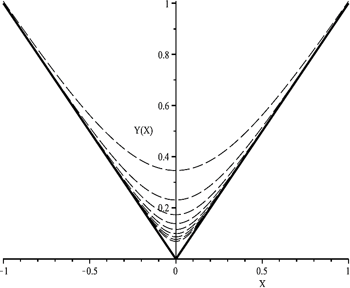
being α = 106 and β = 2.3 appropriate values to achieve small tolerance results. An absolute-value function approximation for α = 4, 6, 8, ..., 20 and β = 2.3 can be observed in Figure 1. In this figure the thin traces (dashed lines) correspond to these approximations while the thickest one corresponds to the exact absolute-value function y(x) = |x|. The thin uppermost curve represents the plot for (α = 4, β = 2.3) and the lowest curve for (α = 20, β = 2.3).
3. Divide the function domain into an equally sized grid. For one-dimensional functions this partition is done by the set of vertical line equations pn(x) = x = i, with i = 1, 2, · ··, (N - 1). For two-dimensional functions the line equations pn(x, y) are constructed by following a simplicial subdivision over the plane XY which is composed of three types of traces: vertical (pn(x, y) = x = i), horizontal (pn(x, y) = y = i), and crosswise (pn(x, y) = x - y = i). Particularly, for each of these traces the sweep of i must be in accordance with the boundaries existing along the X and Y axes. For example, if the restrictions X = s1 and Y = s2 are defined in the XY plane, the sweeps i = {1, 2, ···, (s1 - 1)}, i = {1, 2, ···,(s2 -1)}, and i = {(-s1 + 1), (- s1 + 2), ··· ,0,1, ··· ,(s2 - 1)} will correspond to the horizontal, vertical, and crosswise traces, respectively.
4. Order the vertexes appropriately. This means that the vertexes must be ordered according to their class. For a two-dimensional domain s1 x s2, the class-zero vertex is the point located at the origin of a coordinate system XY, the class-one vertexes are the coordinates (xi , 0) and (0, Yj) (for i = 1, 2,..., s1 and j = 1, 2, ..., s2, respectively) and the set of class-two vertexes is composed by the coordinates (Xi , Yj), with the j-th index running as j = 1, 2, ... , s2 for each i-th value from 1 to s1. Likewise, for a one-dimensional domain X, bounded by a closed interval [s0, s1], only the vertexes class-zero (the coordinate (s0, 0)) and class-one (the coordinates (i, 0) for i = 1, 2, ..., s1) exist.
5. Generate the symbolic basis-functions Λk = γk (pn), with the index k closely dependent on the vertical and horizontal partition line equations. For example, in a two-dimensional domain s1 x s2 will be a set PH of (s1 - 1) horizontal equations, and a set PV of (s2 - 1) equations. If a cartesian product between these sets is formed, then each ordered pair whose first component is an equation member of PH and whose second component is an equation member of PV will be evaluated in the basis-function Λk with k = 0, 1, ..., (s1 -1) x (s2 - 1) . The set of these functions is arranged in vectorial form as
For a one-dimensional domain only vertical line partition equations will be presented and k = 0, 1, 2, ... , (s1 - 1).
6. Evaluate the vector of basis-functions Λ at each ordered vertex. It is important to observe the similarity that exists between the methodology used to order the vertexes and which is used to construct the matrix ΛV constituted by the rows of evaluated vectors Λ:
where n indicates the number of vertexes. For the one-dimensional case, the above procedure is practically the same with the only difference of evaluating two classes of vertexes (zero- and one-, type).
7. Provide the values of function Bi at the breakpoint coordinates by following a sorted order associated with the vertices V0, V1 ,..., Vn . These values are written as follows
This step is indistinctly implemented in the construction of one-dimensional and two-dimensional functions.
4 Simulation Results
In this section, three examples to illustrate the effectiveness of the proposed smoothing strategy are presented. We use the software Maple Release 15 to build the mathematical models and plot the approximate functions.
Example 1: Let the sequence of data points D = {(0,0), (1,2), (2,1), (3,3), (4, -1), (5,5)} be used to determine a smooth-piecewise function ys(x) in the range [0,5] of x. In order to have a comparative reference, the methodology of Pedro-Julian et al.[8] is used to obtain a piecewise-linear function that satisfies the condition of constructing new data points within the range of [0, 5]. As a result, the function y(x) is obtained.
 (9)
(9)
In accordance with the construction methodology presented in the previous section, a smooth function ys(x) can be determined by replacing the γ basis-function by its logarithmic approximation reported in equation (6). With aid of Maple software, the resulting smooth expression can be simplified in a more compact algebraic form as
With
Table 1 Function parameters for the smooth-piecewise function ys(x)
| i | Ai | Bi | Ci | Ei | Gi | Hi | Li | Mi |
| 1,2 | ±0.10687 | -10 | +10 | ±0.43429 | -10 | +10 | +10 | -10 |
| 3,4 | ±0.10687 | +10 | -10 | ∓0.43429 | -10 | +10 | +10 | -10 |
| 5,6 | ±0.13428 | +10 | 0 | ±0.43429 | -10 | 0 | +10 | 0 |
| 7,8 | ±0.13428 | -10 | 0 | ∓0.43429 | -10 | 0 | +10 | 0 |
| 9,10 | ±0.11231 | +10 | -20 | ±0.43429 | -10 | +20 | +10 | -20 |
| 11,12 | ∓0.11231 | -10 | +20 | ±0.43429 | -10 | +20 | +10 | -20 |
| 13,14 | ±0.20782 | -10 | +30 | ±0.43429 | -10 | +30 | +10 | -30 |
| 15,16 | ∓0.20782 | +10 | -30 | ±0.43429 | -10 | +30 | +10 | -30 |
| 17,18 | ±0.30705 | +10 | -40 | ±0.43429 | -10 | +40 | +10 | -40 |
| 19,20 | ±0.30705 | -10 | +40 | ∓0.43429 | -10 | +40 | +10 | -40 |
| 21, 22 | +0.26858 | ±10 | 0 | 0 | 0 | 0 | 0 | 0 |
| 23, 24 | -0.41564 | ∓10 | ±30 | 0 | 0 | 0 | 0 | 0 |
| 25, 26 | +0.22462 | ∓10 | ±20 | 0 | 0 | 0 | 0 | 0 |
| 27, 28 | -0.21375 | ∓10 | ±10 | 0 | 0 | 0 | 0 | 0 |
| 29, 30 | +0.61411 | ∓10 | ±υ40 | 0 | 0 | 0 | 0 | 0 |
In Figure 2 the dashed line shows the curve of the function y(x) while the solid line depicts the curve for the smooth-piecewise function ys(x).
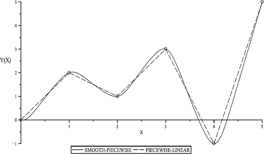
Fig. 2 Function approximation: piecewise-linear (equation (9), dashed line) and smooth-piecewise (equation (10), solid line)
An error between the piecewise-linear function and its smooth version can be estimated by the percent error formulation
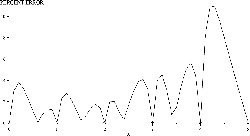
From this figure two important results must be underlined: the error is distributed along each linear segment and a precise fitting is achieved at the breakpoints locations. Moreover, an interesting property can be observed if the differentiability of functions y(x) and ys(x) is put under testing. As can be noted in Figure 4, for the function y(x) only the first order derivative is defined (except in the breakpoints) while the n-order derivative (for all n ≥ 1) is zero or not defined.
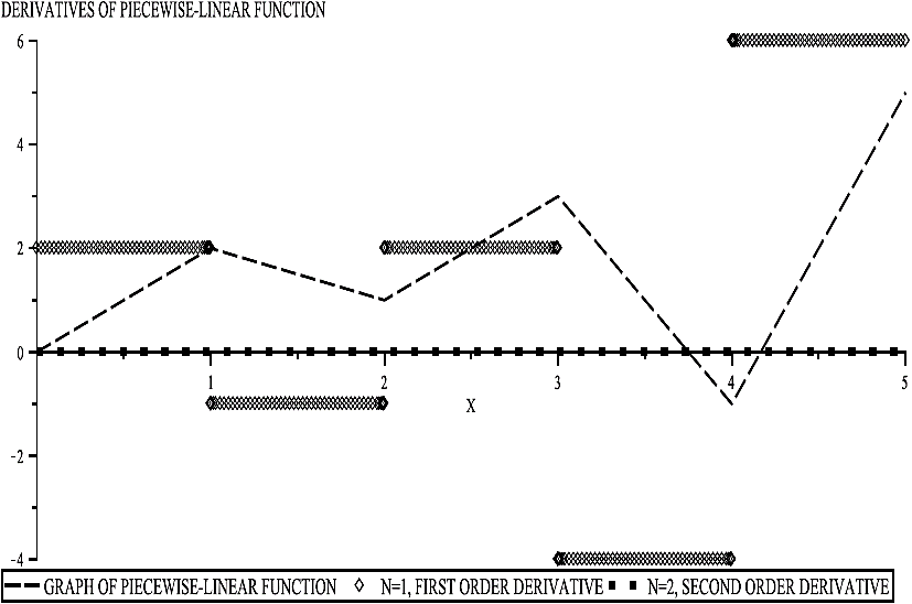
In contrast, it must be noted that the existence of the higher order derivatives is guaranteed in the smooth function due to the fact that its second derivative is continuous everywhere.
As an example, Figure 5 shows curves for the first and second order derivatives of ys(x).

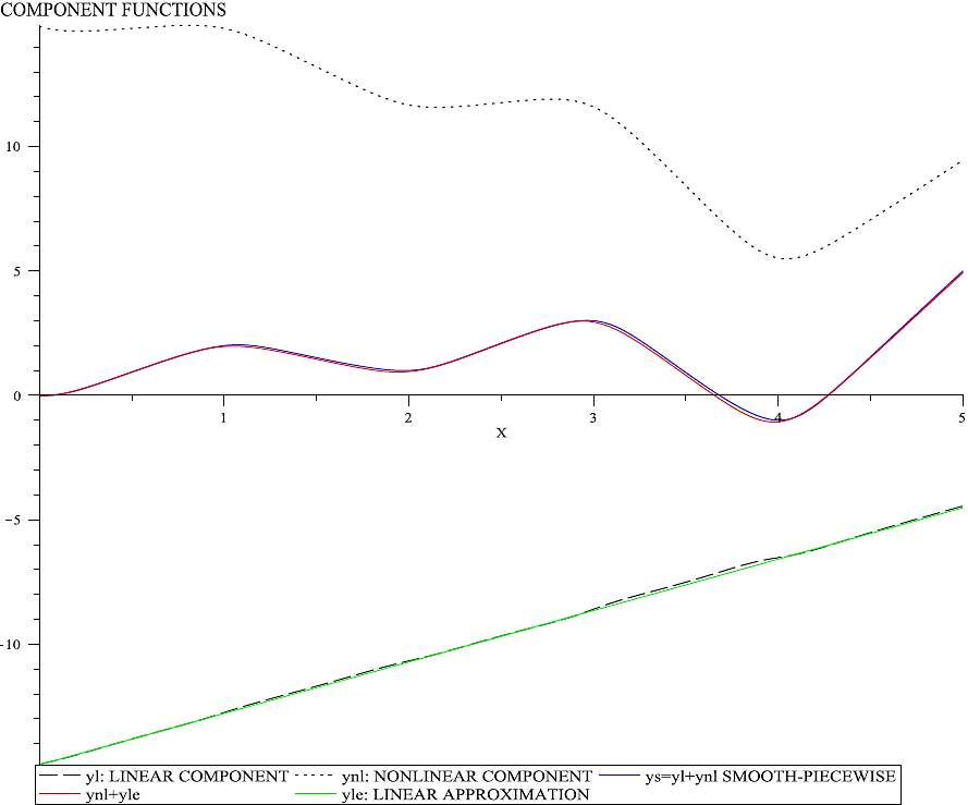
An important observation regarding to equation (10) is that it can be decomposed into two component functions which can be derived from the parameters reported in Table 1: one for i = 1,···,20, denoted as yl(x), and another for i = 21,···,30, expressed as ynl(x). This means that the smooth piecewise function can be expressed as ys(x) = yl(x) + ynl(x), with a nonlinear behavior of the characteristic curve of ys(x) mainly contained in ynl(x), and a quasilinear behavior strongly related to yl(x). This allows to simplify the smooth-piecewise function in a more compact expression by approximating yl(x) with a line equation yle(x) (for this example, yle(x) = 2.0666667x + 14.84611591). As expected, a good approximation of ys(x) is obtained by ynl(x) + yle(x). Considering this result, equation (10) can be expressed (also in reference to Table 1) in a more compact form:
In Figure 6 graphs of ys(x), yl(x), ynl(x), and yle(x) functions are shown.
Example 2: In this example it is assumed that the only input data that is available to construct an interpolation function z (x, y) is the set of points D.
D={(0,0,1),(1,0,0),(2,0,2),(3,0,0),(0,1,0),(0,2,1), (3,3,0),(1,1,0),(1,2,0),(1,3,2),(2,1,1),(2,2,1),(2,3,0), (3,1,0),(3,2,0),(3,1,3)}.
By following the traditional construction methodology of Pedro-Julian et al. 8, a two dimensional piecewise-linear
function
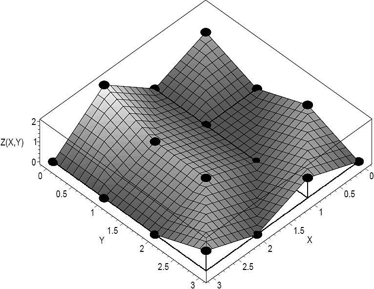
Fig. 7 Surface for the two-dimensional simplicial piecewise-linear function obtained from the input data D of Example 2
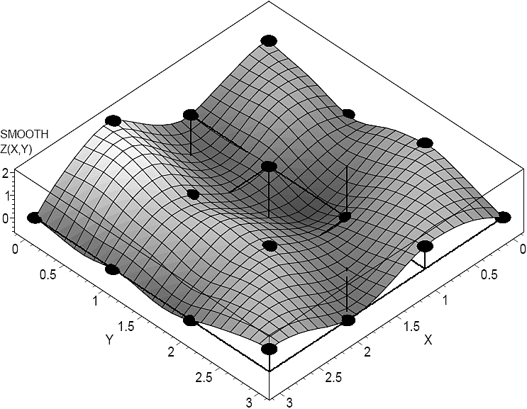
Fig. 8 Surface for the two-dimensional smooth-piecewise function obtained from the input data D of Example 2
Similarly to what was done in the one-dimensional example, a precise curve fitting was achieved at the breakpoint coordinates while the maximum deviation between the curves which are depicted in Figure 7 and Figure 8 is observed inside of each simplex in the XY plane. In Figure 9 this effect can be graphically appreciated. Additionally, it must be observed that in contrast with the original piecewise-linear function where the second and higher order derivatives are null, in the smooth function this problem is overcome. In order to illustrate this numerical advantage, surfaces for the first and second derivative of
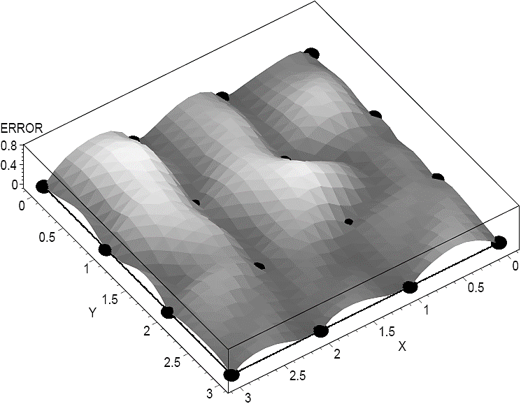
Fig. 9 Deviation between the piecewise-linear and the smooth curve obtained from the input data D of Example 2
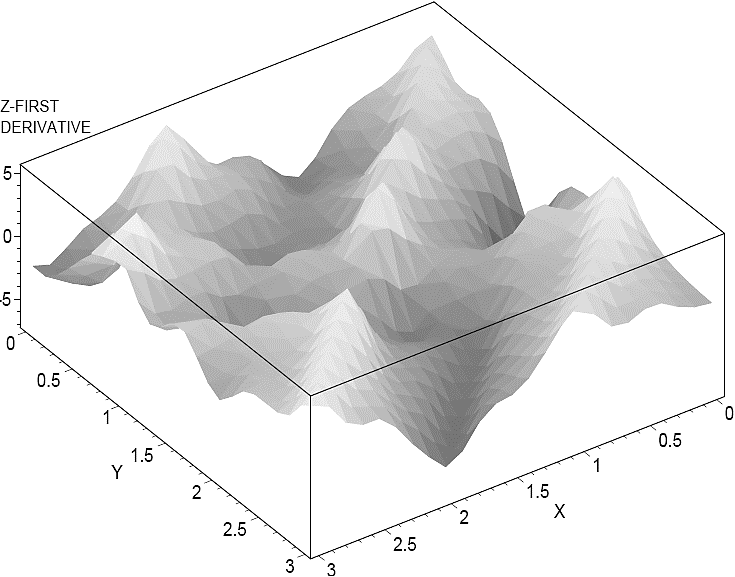
Fig. 10 Derivatives of function
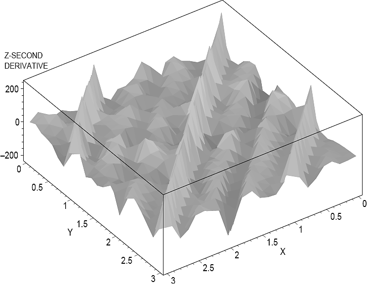
Fig. 11 Derivatives of function
Example 3: This example illustrates a potential application of the smoothing proposal in a typical problem of control systems engineering. The black curve of Figure 12 represents the transient response of a second-order system for a unit-impulse excitation. Consider that we are interested in determining the time tp when the maximum peak of this response occurs. Let us consider that the analytical transfer function is not accessible and only a set of equally spaced breakpoints (discrete measurements) is the input data available to construct an approximate function. By following the construction strategy exposed in section 3, the two approximations depicted in Figure 12 can be obtained: piecewise-linear cpwl(t) (red) and smooth-piecewise cs(t) (blue).
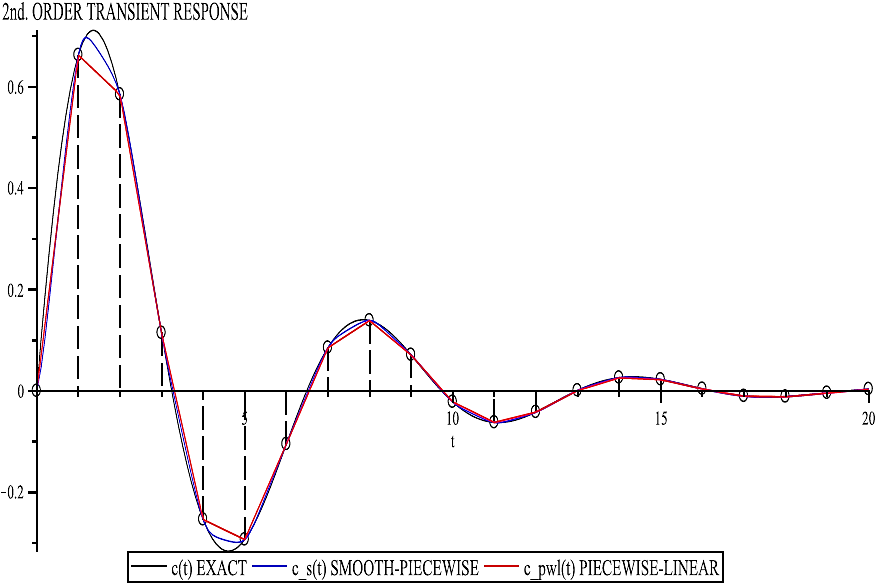
Fig. 12 Approximate functions for the transient response c(t): smooth-piecewise cs(t), piecewise-linear cpwl(t)
In Figure 12, the corresponding smooth and piecewise-linear functions are expressed in the form
and
with the parameters summarized in Table 2 and Table 3, respectively.
Table 2 Function parameters for the piecewise-linear function cpwl(t)
| i | Âi |
|
αi=βi = γi |
| 0 | +0.33134 | -0.16567 | 0 |
| 1 | -0.37020 | +0.18510 | 1 |
| 2 | -0.19642-1 | +0.98210 x 10⁻¹ | 2 |
| 3 | +0.51145 x 10 | -0.25572 x 10⁻¹ | 3 |
| 4 | +0.16428 | -0.82140 x 10⁻¹ | 4 |
| 5 | +0.11400 | -0.57000 x 10⁻¹ | 5 |
| 6 | +0.9960 x 10⁻³ | -0.49800 x 10⁻³ | 6 |
| 7 | -0.68265x 10⁻¹ | +0.34132 x 10⁻¹ | 7 |
| 8 | -0.60870x 10⁻¹ | +0.30435 x 10⁻¹ | 8 |
| 9 | -0.12327x 10⁻¹ | +0.61635 x 10⁻² | 9 |
| 10 | +0.26036 x 10⁻¹ | -0.13018 x 10⁻¹ | 10 |
| 11 | +0.30461 x 10⁻¹ | -0.15230 x 10⁻¹ | 11 |
| 12 | +0.11096 x 10⁻¹ | -0.55482 x 10⁻¹ | 12 |
| 13 | -0.86790x 10⁻² | +0.43395 x 10⁻² | 13 |
| 14 | -0.14392x 10⁻¹ | +0.71962 x 10⁻² | 14 |
| 15 | -0.74405x 10⁻² | +0.37202 x 10⁻² | 15 |
| 16 | +0.21605x 10⁻² | -0.10802 x 10⁻² | 16 |
| 17 | +0.64210x 10⁻² | -0.32105 x 10⁻² | 17 |
| 18 | +0.43571 x 10⁻² | -0.21786 x 10⁻² | 18 |
| 19 | -0.47850x 10⁻⁴ | +0.23925 x 10⁻⁴ | 19 |
Table 3 Function parameters for the smoothing piecewise-linear function cs(t)
| i | Ni | ki |
| 1, 2 | +0.039087 | 0, 0 |
| 3, 4 | -0.044564 | 1, 1 |
| 5, 6 | -0.019685 | 2, 2 |
| 7, 8 | +0.0061166 | 3, 3 |
| 9, 10 | +0.017621 | 4, 4 |
| 11, 12 | +0.011828 | 5, 5 |
| 13, 14 | -0.0002595 | 6, 6 |
| 15, 16 | -0.0073524 | 7, 7 |
| 17, 18 | -0.0064319 | 8, 8 |
| 19, 20 | -0.0010948 | 9, 9 |
| 21, 22 | +0.0028448 | 10, 10 |
| 23, 24 | +0.0031831 | 11, 11 |
| 25, 26 | +0.0011504 | 12, 12 |
| 27, 28 | -0.00098792 | 13, 13 |
| 29, 30 | -0.0015378 | 14, 14 |
| 31, 32 | -0.00077512 | 15, 15 |
| 33, 34 | +0.00027019 | 16, 16 |
| 35, 36 | +0.00072258 | 17, 17 |
| 37, 38 | +0.00039166 | 18, 18 |
| 39, 40 | +0.000014116 | 19, 19 |
From this set of data, we may determine the peak time (tp) by differentiating the approximate function (cpwl(t) or cs(t)) with respect to time (t) and setting this derivative equal to zero
or
However, for the piecewise-linear function a numerical solution cannot be reached, hence the smooth function cs(t) appears as the better approximation alternative. After solving equation (15) with Maple software we obtain tp = 1.193s, which clearly corresponds to the peak time. The piecewise-linear cpwl(t) and the smooth-piecewise cs(t) approximations of the impulse transient response, as well as their derivatives with respect to time, are shown in Figure 13.
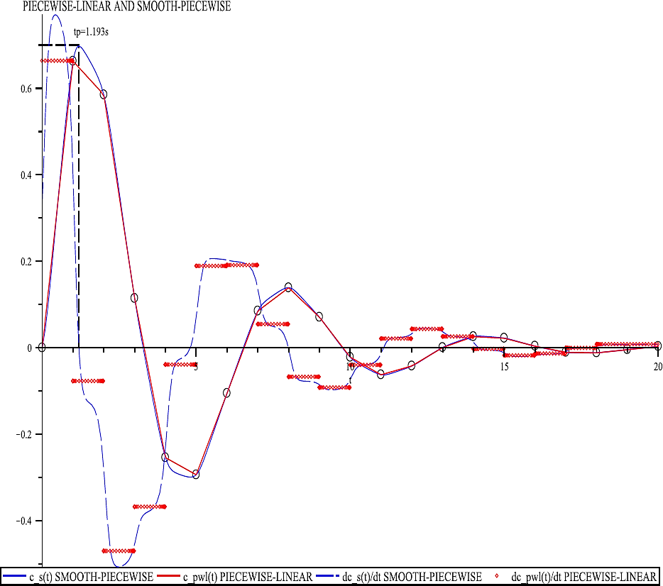
Fig. 13 Approximate functions and derivatives for the transient response: piecewise-linear and smooth-piecewise
In this figure, it is important to observe the notorious difference that exists, from the point of view of function continuity, between the derivatives of these two approximate functions: while
5 Comparative Discussion
In this section, a comparative discussion about the curve fitting performance of the proposed method against other strategies such as polynomial and cubic spline techniques is presented. To start this analysis, it is important to mention that a better curve fitting can be achieved by the smooth-piecewise method, this is because it always imposes on the function the condition of passing through the input data coordinates. Similarly to the piecewise-linear functions, the continuity is also preserved in all the function domain but unlike the piecewise-linear reference, the smoothing proposal adds the function differentiation capability. In contrast, although in polynomial interpolation the function continuity is guaranteed, curve fitting is not very precise what results in a remarkable curve deviation that increases the derivative growing very quickly. An alternative approach to minimizing the curve fitting error is the spline interpolation which consists in restricting the approximation to low degree polynomials (typically, like in our comparative analysis, polynomials of third order degree are preferred) over partitioned sections along the function domain. However, in spite of showing a better curve fitting in comparison to the polynomial counterpart, the best performance is clearly obtained by the smooth-piecewise proposal. To emphasize this characteristic, the smooth-piecewise, polynomial, and spline approximate functions for DC = {(0, 5), (1, 3), (2,10), (3,0), (4, 3), (5,1), (6,10)} are shown in Figure 14.
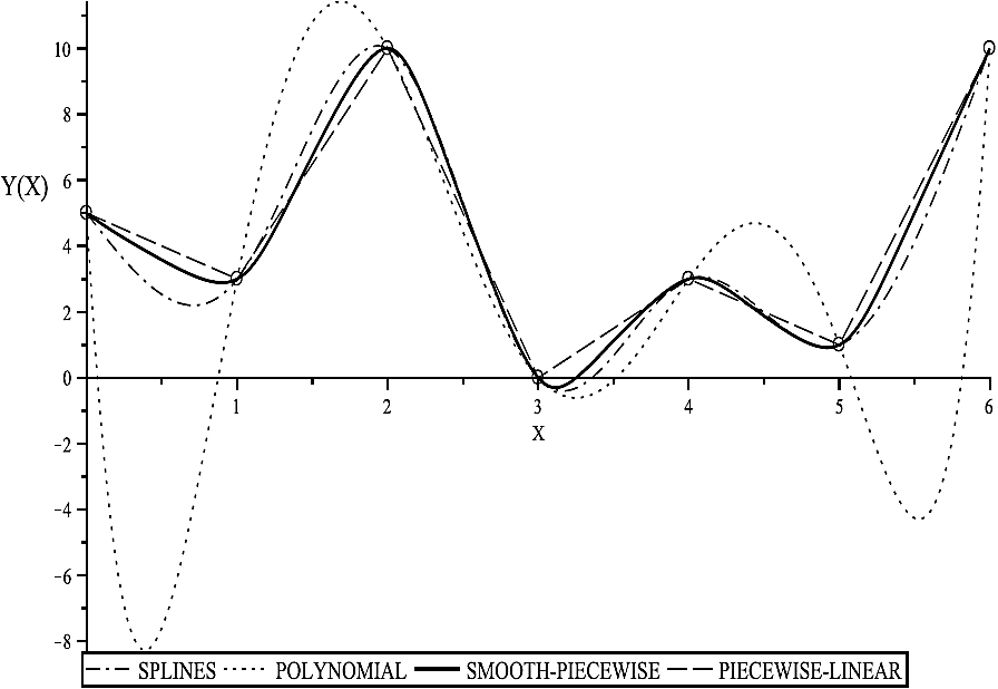
Fig. 14 Approximate functions for the input data Dc: piecewise-linear, smooth-piecewise, polynomial, and splines
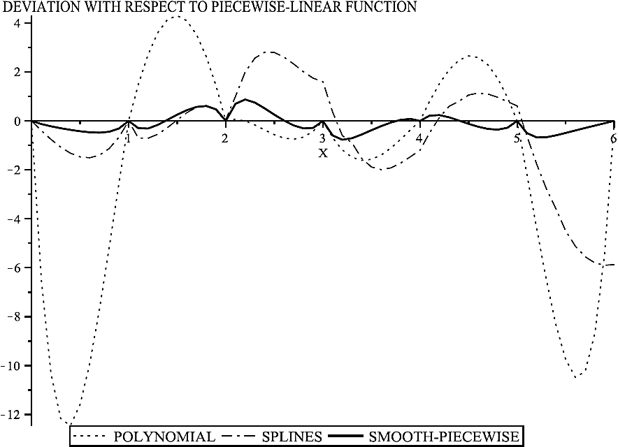
The error in these approximations can be estimated by the deviation e among the smooth-piecewise, polynomial, and splines curves with respect to the piecewise-linear reference. Such deviations are depicted in Figure 15.
6 Conclusion
In this paper, the proof-of-concept related to obtaining smooth-piecewise functions by replacing the basis-function used in the construction methodology of the High Level Canonical piecewise-linear model was demonstrated by numerical simulations. In accordance with such simulations, smooth-piecewise functions not only preserve curve fitting accuracy but also incorporate derivation capability. By illustrative examples, it was observed that the error between the original piecewise-linear curve and its smoothing version is uniformly distributed along each linear partition, being more pronounced approximately before and after its middle location and extremely reduced around the breakpoints. Moreover, two very important observations must be highlighted: the smooth function can be decomposed into two representations (one nonlinear and other quasilinear), and the number of terms of the resulting smooth function can significantly be reduced due to the fact that a great number of them can be approximated by a line equation. Although its potential application to practical engineering problems was illustrated in Example 3, now our ongoing work centers on exploring alternative applications for this smoothing strategy.

