


 nueva página del texto (beta)
 Inglés (pdf)
 Artículo en XML
 Referencias del artículo
 Enviar artículo por email
 Citado por SciELO
  Similares en
SciELO
Similares en
SciELO 
 Permalink
1. Introduction
Trajectory tracking is a well studied problem in control theory. Its applications cover a wide range of topics from recognition of moving objects to synchronization, see, for example, 3, 9, 11 Complex networks are dynamical systems interconnected by a function. Its behavior can be difficult to control and the dynamics of its nodes require a precise analysis, see for example 4. In the classical case, one can track the nodes of the network by using Lyapunov theory and neural networks as in 10.
In recent years, there has been an increasing interest in studying fractional order systems, i.e. dynamical systems with differential equations of fractional order, see, for example, 1. In these systems, the classical mathematical notion of derivative is changed to allow arbitrary orders. Fractional order neural network synchronization is studied, for instance, in 6. In the case of complex dynamical networks of fractional order, cluster synchronization, stabilization, and partial synchronization has been studied, see 7, 8, 5.
In this paper we propose to use recurrent neural networks to track the nodes of a fractional order complex network. We use a Lyapunov function and the result in 2 to design a control law that tracks the system. We prove that tracking is guaranteed by showing that the error between the network and the neural network stabilizes if the control is applied. We show this in a rigorous mathematical form. The control law we obtain is of very general nature and applies to general networks. We provide an example to show how the control law applies to a specific situation.
2. Mathematical Models
2.1 Fractional General Complex Dynamical Network
In this work we use Caputo’s fractional operator which is defined, for 0 < α <1, by
If x(t) ∈ ℝn, we consider that x(α)(t) is the Caputo fractional operator applied to each entry:
Consider a network consisting of N linearly and diffusively coupled nodes, with each node being an n-dimensional dynamical system, described by
where xi = ( xi1, xi2,…, xin )T ∈ ℝn are the state vectors of node i, fi : ℝn ↦ ℝn represents the self-dynamics of node i, constants cij > 0 are the coupling strengths between node i and node j, with i, j = 1, 2,…, N. Γ= (τij ) ∈ ℝn × n is a constant internal matrix that describes the way of linking the components in each pair of connected node vectors (xj - xi ): i.e. for some pairs (i, j) with 1 ≤ i, j ≤ n and τij ≠ 0 the two coupled nodes are linked through their ith and jth sub-state variables, respectively, while the coupling matrix A = (aij) ∈ ℝN × N denotes the coupling configuration of the entire network: i.e. if there is a connection between node i and node j(i ≠ j), then aij = aji = 1; otherwise aij = aji = 0.
2.2 Fractional Recurrent Neural Network
Consider a fractional recurrent neural network in the following form:
where
3 Trajectory Tracking
The objective is to develop a control law such that the ith fractional neural network (2) tracks the trajectory of the ith fractional dynamical system (1). We define the tracking error as ei = xin - xi, i = 1, 2, …, N whose time derivative is
From (1), (2) and (3), we obtain
Adding and substrating Winσ(xi), αi(t), i = 1, 2, …, N, to (4), where αi is defined below, and considering that xin = ei + xi , i = 1, 2, …, N, then
In order to guarantee that the ith neural network (2) tracks the ith reference trajectory (1), the following assumption has to be satisfed:
Assumption 1. There exist functions ρi (t) and αi(t), i =1, 2, …, N, such that
Let’s define
From (6) and (7), equation (5) is reduced to
We can also write
where we used cinjn = cij and ainjn = aij . Then, with the above equation, equation (8) becomes
It is clear that ei = 0, i = 1, 2, …, N is an equilibrium point of (10), when ũin = 0, i = 1, 2, …, N. Therefore, the tracking problem can be restated as a global asymptotic stabilization problem for the system (10).
4 Tracking Error Stabilization and Control Design
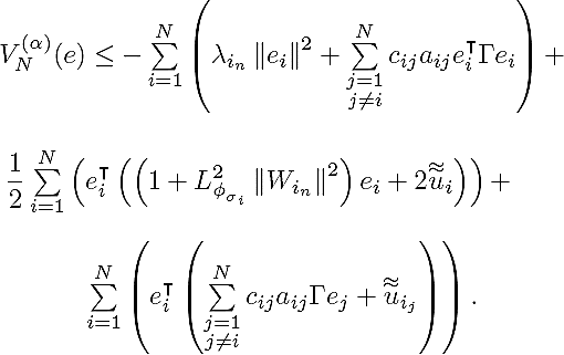
In order to establish the convergence of (10) to ei = 0, i = 1, 2, …, N, which ensures the desired tracking, first, we propose the following candidate Lyapunov function
In fractional calculus, the product rule for the derivative is no longer valid. However, we still have an upper bound for the product that appears in (11). Specifically, from Lemma 1 in 2 the time derivative of (11), along the trajectories of (10), is
We can then write

 (13)
(13)
Next, let’s consider the following inequality, proved in 12:
which holds for all matrices X, Y ∈
ℝn×k and Λ ∈
ℝn×n with
Λ = Λ⊤ > 0. Applying (14) with Λ =
ln×n to the
term
Since ϕσ is Lipschitz, then
with Lipschitz constant
Next, (15) is reduced to
Then, we have that
 (19)
(19)
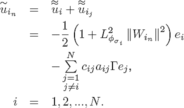
We define
 (20)
(20)
Now, we propose to use the following control law:
 (21)
(21)
In this case,
Finally, the control action of the recurrent neural networks is given by
 (22)
(22)
5 Simulations
In order to illustrate the application of the discussed results, we consider a simple network with four different nodes and five non-uniform links, see Fig.1. The node self-dynamics are described by (see 13 for the origins of this example):
 (23)
(23)
and the coupling strengths are c12 = c21 = 1.3, c14 = c41 = 1.0, c13 = c31 = 2.7, c24 = c42 = 2.1, c34 = c43 = 1.5.
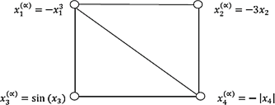
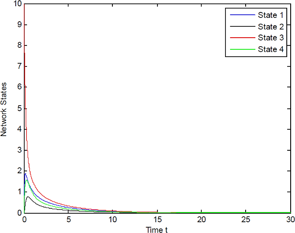
Fig. 2 shows the divergent phenomenon of network (23) with initial state X(0) = (0,0,10,0)T and a three-time stronger coupling strength.
The neural network was selected as
with initial state xn(0) = (0,0,-10,0)T and Γ = I1×1.
The simulation was as follows: for the first 0.5 seconds, the two systems evolve by themselves; in this moment the control law (22) is applied.
Figure 3 represents numerical solutions of the following: 1) the dynamical system of integer order for the first state of the complex network (called original state in the figure), 2) the corresponding integer order neural network (called original state in the figure), 3) the dynamical system of fractional order for the first state, 3) the corresponding neural network.

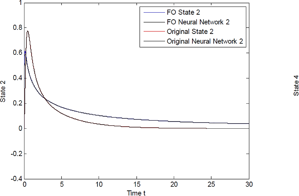
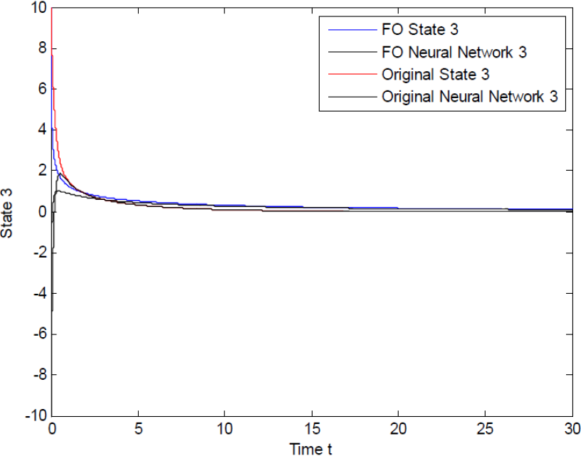
Similar results for states 2, 3 and 4 are displayed in Fig. 4, Fig. 5, and Fig. 6, respectively. They show the time evolution for network states and the successful tracking as was expected from the general control law we obtained.

6 Conclusions
We have presented a controller design for trajectory tracking of a fractional general complex dynamical networks 15. This framework is based on controlling dynamic neural networks using Lyapunov theory in the fractional case. We obtained a control law in a purely theoretical way, and it can be applied to a wide range of problems in trajectory tracking. As an example, the proposed control is applied to a simple network with four different nodes and five non-uniform links. In future work, we will consider the stochastic case in fractional systems.

