


 nova página do texto(beta)
 Inglês (pdf)
 Artigo em XML
 Referências do artigo
 Enviar este artigo por email
 Citado por SciELO
  Similares em
SciELO
Similares em
SciELO 
 Permalink
1 Introduction
A simple method to classify patterns provides the probability of class membership based on evaluating linear functions on a set of predictive variables. However, quite often, in real-world classification problems, we cannot assume linearity in input variables. Specifically, in this paper we analyze an algorithm that avoids the effects of non-linearity of the input variables. Using an approach based on non-linear functions constructed with the product of the inputs raises to arbitrary powers. The exponents are real values and can be adjusted by machine learning. These functions can discover relations between predictive variables. The Product-Unit based Neural Networks (PUNN) were introduced by Durbin and Rumelhart in 9. They are an alternative to sigmoidal neural networks and are based on multiplicative nodes instead of additive ones. Their training is more difficult than the training of standard sigmoidal-based networks. The cause is the existence of multiple local optima and plateaus in the error surface. The main reason for this difficulty is that small changes in the exponents can cause large changes in the total error surface. The complexity of the error surface associated with PUNN justifies the use of an evolutionary algorithm to design the topology of the network and to train its corresponding weights. In this case PUNN becomes EPUNN. This novel approach has been subjected to few comparisons in different scopes since its invention by Martínez-Estudillo et al. 16. For this reason we compared the Evolutionary Product-Unit Neural Network Classifier (EPUNN) with some of the top ten 26 classifiers: NB, SVM, KNN, and C4.5 in four different comparative scenarios: noisy data, imbalanced data, missing values data sets, and classical data sets. In section [section:EPUNN] we describe in detail the main characteristics of the EPUNN classifier and in section [section:related:work] we describe the remaining algorithms.
With this work, we have made the following contributions: we validated experimentally (in 21 classical data sets) that EPUNN behaves similarly to four of the top ten algorithms; we showed that its performance is greatly reduced (exponentially), when the level of noise present in the data sets increases; we found that its performance is better than the performance of the others algorithms on imbalanced data sets; finally, EPUNN decreases its performance when executed on data sets with missing values (see details about the data sets in section 4.1).
The methodology for the evaluation can be consulted in section 4, the tools are presented in section 4.2, and the statistical analysis is given in section 4.3.
2 Evolutionary Product-Unit Neural Networks Classifiers
The method consists of obtaining the neural network architecture and simultaneously estimating the weights of the model coefficients with an algorithm of evolutionary computation. A cross-entropy error function is used in the neural model. In this way a neuro-evolutive model is obtained from the training set and then checked against the patterns of the testing set. Some advantages of Product-Unit Neural Networks (PUNN) are their increased information capacity and the ability to form higher-order combinations of inputs. In the early work of Durbin and Rumelhart 9 it was determined empirically that the information capacity of product units (learning random boolean patterns) is approximately 3N, compared to 2N of a network with additive units for a single threshold logic function, where N denotes the number of inputs to the network. Despite these advantages, product-unit based networks have a major drawback: they have more local optima and more probability of becoming trapped in them 12. The main reason for this difficulty is that small changes in the exponents can cause large changes in the total error surface and therefore their training is more difficult than the training of standard sigmoidal based networks. Several efforts have been made to carry out learning methods for product units 12, 10. Studies carried out on PUNN have not tackled the problem of designing the structure and weights simultaneously in this kind of neural network, either using classic or evolutionary methods.
In this type of algorithm it is not possible to work with inputs that have negative values. Because weights are often non-integer values, therefore there would be roots of negative numbers which result in complex numbers. Since neural networks with complex outputs are rarely used in applications, Durbin and Rumelhart suggested discarding the imaginary part and using only the real component for further processing but this manipulation would have disastrous consequences. To avoid this problem, the input domain is restricted. We define the input set by
In 17, 16 a neural architecture was proposed shown in Figure 1, an input layer with n nodes, a hidden layer with m nodes, and an output layer with l nodes, one for each class. The activation function of the j-th node in the hidden layer, hj , is given by equation 1; where wji is the weight of the connection between input node i and hidden node j:
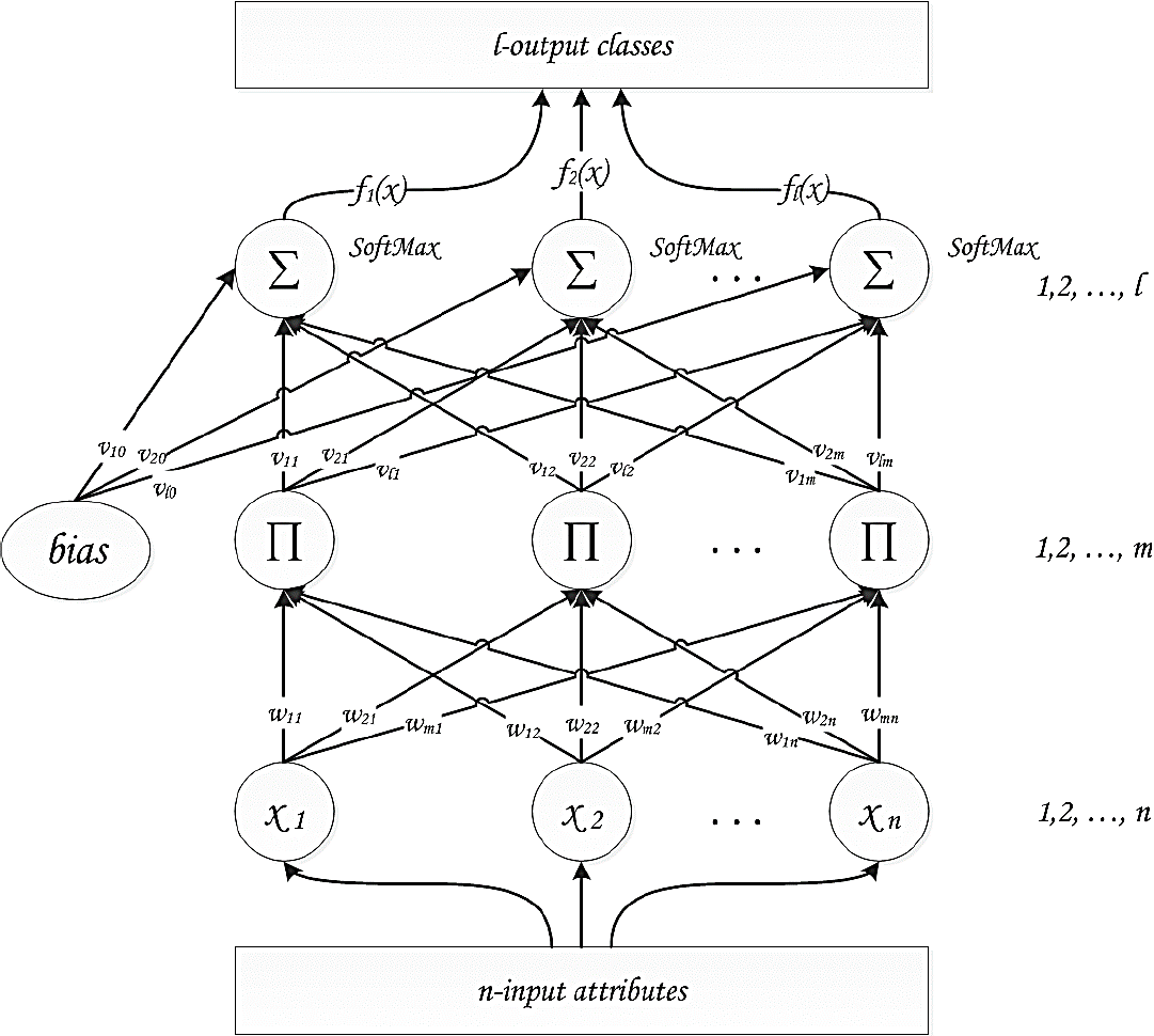
The activation function of the k-th node in the output layer, gk , is given by equation 2 where υkj is the weight of the connection between hidden node j and output node k:
By default the transfer function of all hidden and output nodes is the identity function. In this way, the estimated function gk from each output k=1, 2, …, l, is given by the equation 3:
2.1 Evolutionary PUNN
The authors of 17, 16 applied an evolutionary neural network algorithm to learn the weights that minimize the cross-entropy error function and design the structure of PUNN. The search begins with an initial population of PUNN, and in each iteration the population is updated using a population-update algorithm. The population is evolved by replication and mutation. The authors exclude the crossover operator due to its potential disadvantages suggested by 27, 18 in evolving artificial networks. The pseudo-code of an Evolutionary Product-Unit Neural Network (EPUNN) is shown in (Algorithm 1).
2.2 Classification with EPUNN
A classification problem starts with feature measurements xi,
i = 1, 2, …, n for any single individual
(or object), then the individuals should be classified into one of the
l classes based on these feature measurements. A training
sample D = {(xt ,
xt ); t = 1, 2,…,
T} is available, where xt =
x1t ,
x2t , …,
xnt is the vector of feature measurements
taking values in ψ ⊂ ℜn , and
yt is the class value of the t-th
individual. Based on the training sample we intend to find a decision function
C: ψ → {1, 2, …, l} for
classifying individuals. A misclassification occurs when a decision rule
ψ assigns an individual (based on the feature measurement
vector) to a class k when it actually comes from a class
q ≠ k, where k,
q = 1, 2, …, l. The authors of EPUNN
defined the corrected classification rate (CCR) by
Observe that SoftMax transformation produces positive estimates that sum to one and, therefore, the outputs can be interpreted as the conditional probability of class membership. In general, the parameters needed for operation of the algorithm are given in the next subsection 2.3.
2.4 EPUNN Properties
This model was designed for operation under the following conditions:
- Continuous Variables: true.
- Nominal Variables: true.
- Discretized Variables: true.
- Integer Variables: true.
- Variables without values for some examples: true2
- Variables with imprecise values for some examples: false.
3 Related Work
In this article, we compared the competence of the EPUNN with four widely-known techniques for classification task. More specifically, we compared it with C4.5 20, NB 15, 13, 8, KNN 11, 6, 24, and SVM 5. The KEEL platform was used for all of them.
3.1 C4.5
This algorithm induces classification rules in the form of decision trees from a set of given examples. The decision trees are constructed top-down. In each step a test for the actual node is chosen (starting with the root node), which best separates the given examples into classes. C45 is an evolution of ID3 algorithm 19. The extensions or improvements of ID3 are that it accounts for unavailable or missing values in data, it handles continuous attribute value ranges, chooses an appropriate attribute selection measure (maximizing information gain), and it prunes the result decision trees with minimal description length principle 21.
3.1.1 C4.5 Parameters
This model must be configured in KEEL with the following parameters:
- Prune: allows activating or deactivating the pruning mechanism of the tree.
- Confidence: defines the minimal confidence that a leaf must have in order to be considered in the tree.
- minItemsets: defines the minimum number of instances per leaf. It is an integer value that determines how many data instances must be contained in a leaf in order for the leaf to be created.
3.2 NB
The NB classifier is based on Bayes’ theorem, assuming independence between predictor attributes. The conditional probability of every example to be in a class is computed. Then the output class of the example will be assigned as the highest conditional probability calculated. A Naive Bayesian model is easy to build, with no complicated iterative parameter estimation which makes it particularly useful for very large data sets. Despite its simplicity, the NB classifier often performs surprisingly well (even when it is not known if there is independence between predictor attributes) and it is widely used because it often outperforms more sophisticated classification methods.
3.2.1 NB Parameters
This model must be configured in KEEL without parameters; however, we utilized uniform frequency discretization 14 prepossessing to convert numerical attributes (real and integers) to nominal ones.
3.3 KNN
This is a supervised classification method that permits to estimate the density function of predictive attributes for each class. This estimation is obtained from the information provided by a set of k nearest neighbors. One point in the space is assigned to the class-C if this is the most frequent class between the k nearest examples in the training set. A special case is k =1, in this case the algorithm is known as the Nearest Neighbor Algorithm 6. The Euclidean distance is commonly used as a distance metric.
3.3.1 KNN Parameters
This model must be configured in KEEL with the following parameters:
-K: the number of neighbors to be tested. If this value is too high (similar to the data size), then it is the majority class classifier. When k=1, then it is the nearest neighbor algorithm.
-Distance Function: KEEL-KNN implements tree distance functions:
-Euclidean, with normalized attributes.
-Heterogeneous Value Difference Metric (HVDM) ; this distance function uses the Euclidean distance for quantitative attributes and the VDM distance 22 for qualitative attributes. The VDM metric considers the classification similarity for each possible value of a qualitative attribute to calculate the distances between these values.
-Manhattan, the distance between two points is the sum of the absolute differences of their coordinates.
3.4 SVM
An SVM performs classification by finding the hyperplane that maximizes the margin between two classes. The vectors (instances) that define the hyperplane are the support vectors. The algorithm begins with defining an optimal hyperplane (maximizing the margin). Then the data is mapped to a high dimensional space by means of a Kernel function, where it is easier to classify with linear decision surfaces: the problem is reformulated so that data is mapped implicitly to this space. In the ideal case SVM should produce a hyperplane that completely separates the instances into two non-overlapping classes. However, perfect separation may not be possible, or it may result in a model with so many cases that the model does not classify correctly. Hence SVM finds the hyperplane that maximizes the margin and minimizes the misclassifications. This method is also apt to classify problems with more than two classes with a voting scheme.
3.4.1 SVM Parameters
This model must be configured in KEEL with the following parameters:
- KernelType: which kernel will be used to transform the data.
- C: cost; it is the penalty parameter of the error term.
- Degree: sets degree in kernel function.
- Gamma: sets gamma in kernel function.
- Coef0: sets coef0 in kernel function.
- Shrinking: reduces the size of the optimization problem without considering some bounded variables. The decomposition method then works on a smaller problem which is less time-consuming and requires less memory.
3.4.2 SVM Properties
This model was designed for operation under the following conditions:
- Continuous Variables: true.
- Nominal Variables: false.
- Discretized Variables: true.
- Integer Variables: true.
- Variables without values for some examples: true.
- Variables with imprecise values for some examples: true.
A more detailed description, performance evaluation, and review of current and further research of the four algorithms that we selected for this work can be found condensed in a survey paper 26. They are recognized by the research community as ones of the most influential algorithms for data mining in the classification task.
4 Empirical Evaluation
In this section, we present the experimental methodology followed to evaluate the algorithms presented. In order to undertake the evaluation process, we performed four experiments. In the first one, we compared the performance of the EPUNN algorithm against the others using the accuracy metric. In this case, the evaluation was performed on 21 real-world data sets, in subsection 4.1.1 we present the main features of them. The second experiment was conducted by executing the algorithm EPUNN compared with the others on 11 data sets that were generated with different noise levels. The accuracy was used again as the evaluation metric in this case. Details of how these data sets were generated can be found in subsection 4.1.2. The third experiment was conducted to study the behavior of all algorithms under analysis on a series of data sets with different levels of imbalance, in subsection 4.1.3 we present the main features of them. In this case, as an evaluation metric, the well-known area under ROC curve (AUC) was used, following the recommendations of 23. Finally, we conducted the fourth experiment where we evaluated the behavior of the EPUNN accuracy on several data sets with missing values, the characteristics of these can be viewed in subsection 4.1.4. In what follows, we present the real-world problems chosen for the experimentation, the experimental tools and configurations parameters for each tool, the experimental results, and the statistical analysis applied to compare the obtained results.
4.1 Training Sets
4.1.1 Classical Real-World Training Sets
To perform the first experiment and evaluate the behavior of the EPUNN classifier, 21 real-world data set were chosen from the KEEL repository 1. KEEL is an open source Java software tool which empowers the user to assess the behavior of evolutionary learning and Soft Computing based techniques; in particular, the KEEL-dataset includes the data set partitions in the KEEL format for using regression, clustering, multi-instance, imbalanced classification, multi-label classification, etc. The experiments were executed on the following data sets: appendicitis, australian, automobile, balance, banana, bands, breast, bupa, ecoli, glass, heart, hepatitis, ionosphere, iris, lymphography, pima, sonar, wdbc, wine, wisconsin, and zoo. A summary of the characteristics of these data sets can be seen in Table 1.
Table 1 Data sets characteristics
| Data set | Instances | Atributes | Class |
| appendicitis | 106 | 9 | 2 |
| australian | 690 | 14 | 2 |
| automobile | 159 | 25 | 6 |
| balance | 625 | 4 | 3 |
| banana | 5300 | 2 | 2 |
| bands | 365 | 19 | 2 |
| breast | 277 | 9 | 2 |
| bupa | 345 | 6 | 2 |
| ecoli | 336 | 7 | 8 |
| glass | 214 | 9 | 7 |
| heart | 270 | 13 | 2 |
| hepatitis | 80 | 19 | 2 |
| ionosphere | 351 | 33 | 2 |
| iris | 150 | 4 | 3 |
| lymphography | 148 | 18 | 4 |
| pima | 768 | 8 | 2 |
| sonar | 208 | 60 | 2 |
| wdbc | 569 | 30 | 2 |
| wine | 178 | 13 | 3 |
| wisconsin | 683 | 9 | 2 |
| zoo | 101 | 17 | 7 |
4.1.2 Led Data Sets
In order to obtain several data sets for the second experiment, we utilized the led generators from the UCI3 repository 3. With the parameters shown in Table 2, 11 data sets were generated with 512 instances in each one and with noise from 0 to 50.
Table 2 Led generator parameters
| Data set | # Instances | Seed | % Noise |
| led7-i512-n00 | 512 | 12345678 | 0 |
| led7-i512-n05 | 512 | 12345678 | 5 |
| led7-i512-n10 | 512 | 12345678 | 10 |
| led7-i512-n15 | 512 | 12345678 | 15 |
| led7-i512-n20 | 512 | 12345678 | 20 |
| led7-i512-n25 | 512 | 12345678 | 25 |
| led7-i512-n30 | 512 | 12345678 | 30 |
| led7-i512-n35 | 512 | 12345678 | 35 |
| led7-i512-n40 | 512 | 12345678 | 40 |
| led7-i512-n45 | 512 | 12345678 | 45 |
| led7-i512-n50 | 512 | 12345678 | 50 |
4.1.3 Imbalanced Data Sets
To perform the third experiment and evaluate the behavior of the EPUNN classifier, 16 imbalanced data sets were chosen from the KEEL repository 1. In this case the experiments were executed with the following data sets: glass1, ecoli-0_vs_1, pima, iris0, glass0, glass-0-1-2-3_vs_4-5-6, ecoli1, ecoli2, glass6, ecoli3, ecoli4, glass-0-1-6_vs_5, glass2, glass4, glass5, and ecoli-0-1-3-7_vs_2-6. The first ten data sets have an imbalance ratio less than 9, and the last six, a ratio greater than 9, see Table 3.
4.1.4 Missing Values Data Sets
To perform the fourth experiment and evaluate the behavior of the EPUNN classifier, 10 missing values data sets were chosen from the KEEL repository 1. In this case the experiments were executed with the following data sets: australian+mv, ecoli+mv, iris+mv, pima+mv, wine+mv, automobile-mv, bands-mv, breast-mv, hepatitis-mv, and wisconsin-mv, see Table 4. The first five data sets are used for standard classification with induced missing values.
4.2 Experimental Tools
The experiments were done with the KEEL framework 1. For the experimental executions we used an Intel Core i3-2350M, 2300 MHz dual processor, with 6 GB of RAM, and Ubuntu 12.10 with Linux kernel 3.5.0-46 as the operating system. For each algorithm, we used the default KEEL configurations, except for the case of KNN where we set a value of k = 5.
4.3 Statistical Analysis
We followed the recommendations pointed out by Demšar 7 to perform the statistical analysis of the results in experiments 1 and 3. As suggested by him, we used non-parametric statistical tests to compare the accuracies of the models built by the different learning systems. To compare multiple learning methods, first, we applied a multi-comparison statistical procedure to test the null hypothesis that all the learning algorithms obtained the same results on average. Specifically, we used the Friedman’s test. When the Friedman’s test rejected the null hypothesis, we applied post-hoc Bonferroni-Dunn test and Holm’s step-up step-down procedure.
4.4 Experimental Results
4.4.1 Experiment #1
In the first experiment we evaluated the performance of all the models with the accuracy metric (the proportion of correct classifications on previously unseen examples). We used a ten-fold cross validation procedure with 5 different random seeds over each data set. The average values of the results for each collection are shown in Table 5. The last row shows the average rank of each algorithm. As it can be seen, EPUNN-C is the KEEL implementation of EPUNN algorithm.
Table 5 Accuracy of the algorithms on the classic data sets
| Data set | NB-C | C45-C | KNN-C | SVM-C | EPUNN-C |
| appendicitis | 84.27 (4) | 83.27 (5) | 85.91 (3) | 87.91 (1) | 86.09 (2) |
| australian | 86.67 (1.5) | 85.22 (4) | 84.78 (5) | 85.80 (3) | 86.67 (1.5) |
| automobile | 67.95 (2) | 80.93 (1) | 56.54 (5) | 61.97 (3) | 58.38 (4) |
| balance | 91.20 (3) | 76.80 (5) | 86.24 (4) | 91.68 (2) | 96.16 (1) |
| banana | 71.17 (4) | 89.08 (2) | 89.11 (1) | 55.17 (5) | 74.45 (3) |
| bands | 70.50 (1) | 64.99 (5) | 68.46 (4) | 69.46 (2) | 69.24 (3) |
| breast | 74.40 (2) | 76.92 (1) | 72.28 (4) | 70.75 (5) | 72.93 (3) |
| bupa | 61.16 (5) | 67.00 (3) | 61.31 (4) | 70.14 (2) | 72.76 (1) |
| ecoli | 81.56 (1) | 79.47 (3) | 81.27 (2) | 75.92 (5) | 76.82 (4) |
| glass | 69.28 (1) | 67.44 (2) | 66.85 (3) | 62.59 (5) | 64.40 (4) |
| heart | 82.22 (2) | 78.15 (5) | 80.74 (4) | 84.44 (1) | 81.85 (3) |
| hepatitis | 84.83 (2) | 84.00 (3) | 86.27 (1) | 83.56 (4) | 80.36 (5) |
| ionosphere | 88.90 (3) | 90.90 (2) | 85.17 (5) | 88.03 (4) | 92.30 (1) |
| iris | 94.67 (5) | 96.00 (3) | 96.00 (3) | 96.67 (1) | 96.00 (3) |
| lymphography | 85.76 (1) | 74.30 (5) | 79.44 (4) | 83.98 (2) | 81.30 (3) |
| pima | 74.88 (3) | 74.23 (4) | 73.06 (5) | 77.10 (1) | 76.71 (2) |
| sonar | 77.38 (2) | 70.07 (5) | 83.10 (1) | 77.26 (3) | 74.90 (4) |
| wdbc | 94.38 (4) | 94.55 (3) | 96.83 (1.5) | 94.37 (5) | 96.83 (1.5) |
| wine | 96.05 (1.5) | 94.90 (4) | 96.05 (1.5) | 94.38 (5) | 96.01 (3) |
| wisconsin | 97.67 (1) | 95.63 (5) | 96.95 (2) | 96.51 (3) | 96.36 (4) |
| zoo | 94.47 (3) | 92.81 (5) | 93.64 (4) | 96.50 (1) | 95.89 (2) |
| Rank | 2.4762 | 3.5714 | 3.1905 | 3.0000 | 2.7619 |
According to the results obtained, see Table 5, we statistically analyzed the results to detect significant differences in the accuracy of the obtained models by the different learning methods. The multi-comparison Friedman’s test did not reject the null hypotheses that all the systems performed the same on average with p = 0.1631. The obtained pvalue > 0.05 shows that there does not exist a significant difference between the five algorithms under study. Using an α = 0.10 in equation 5 with k, the number of algorithms, qα = 2.241, and N, the number of data sets, a critical difference of 1.0935 was obtained:
Figure 2 shows the results of Bonferroni-Dunn test, comparing all systems by means of accuracy. The major advantage of this test is that it seems to be easier to visualize because it uses the same critical difference for all comparisons 7.
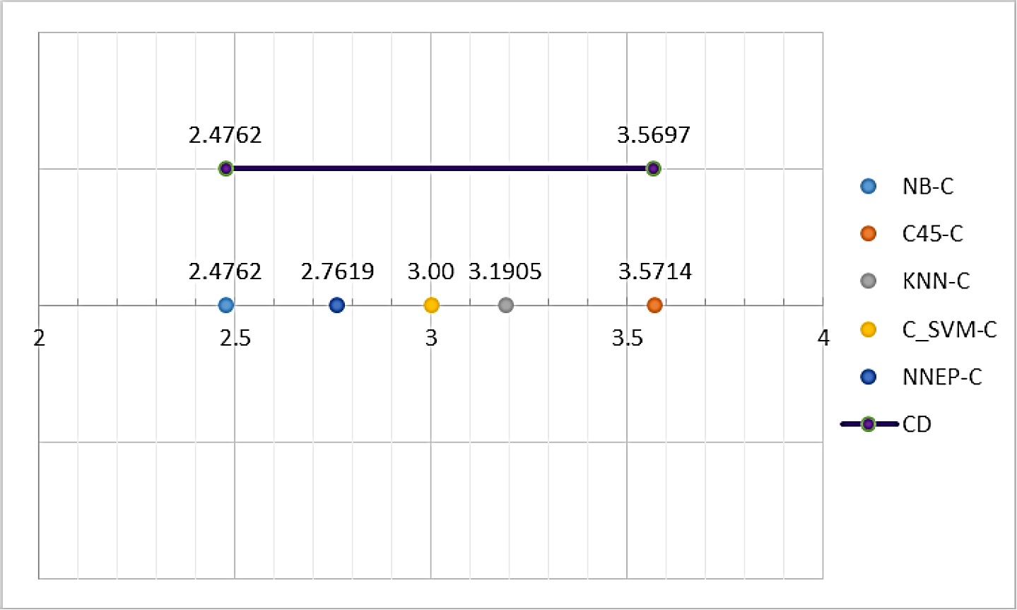
The EPUNN algorithm behaves similarly to four of the top ten algorithms, because its performance is within the critical difference, see Figure 2.
4.4.2 Experiment #2
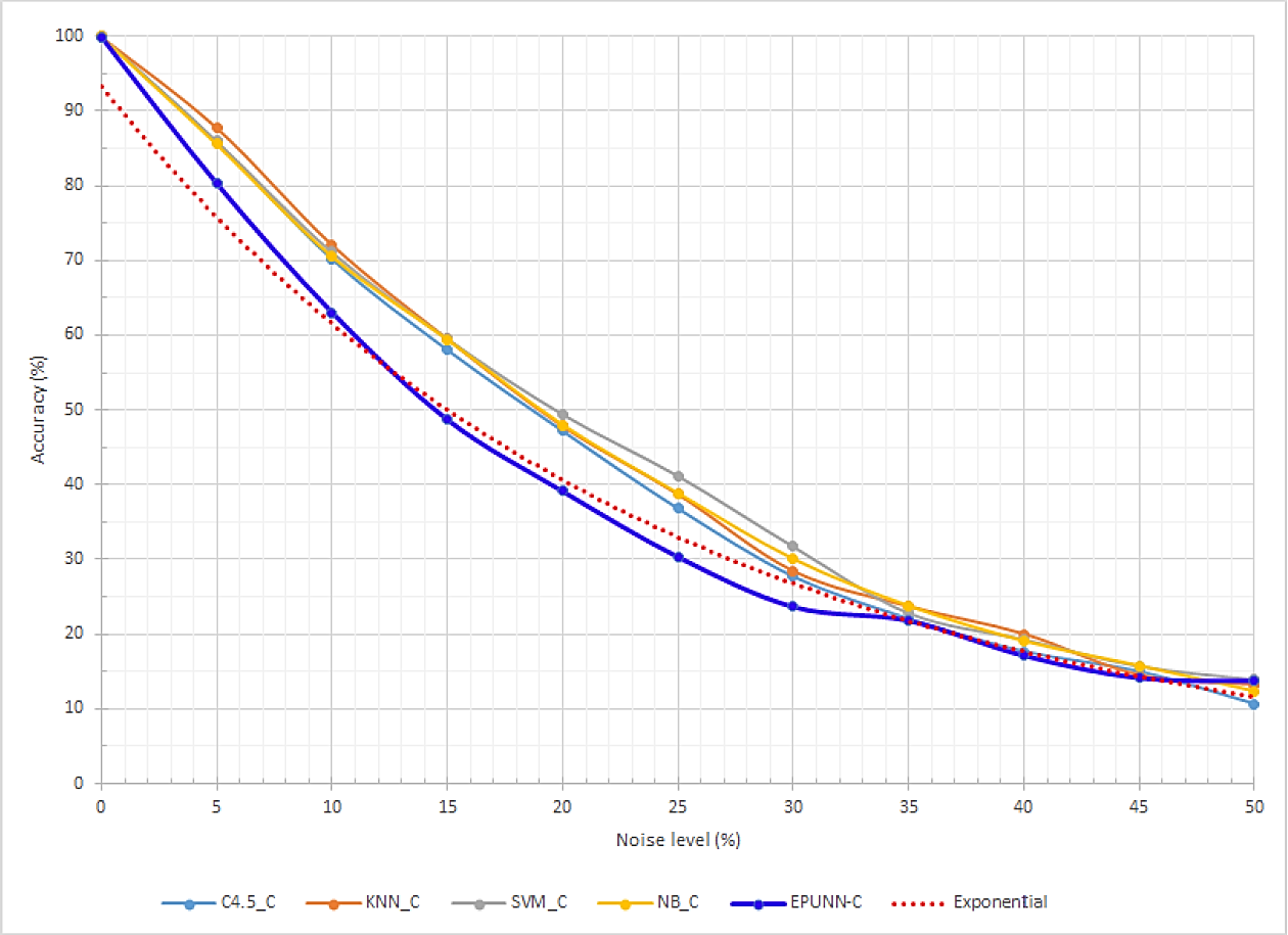
In the second experiment we evaluated the performance of all models in the presence of noise with the accuracy metric. We used a ten-fold cross validation procedure with 5 different random seeds over each data set. The average values of the results for each collection are shown in Table 6.
Table 6 Accuracy of algorithms in the presence of incremental noise in led7 data set
| Data set | % Noise | C4.5-C | KNN-C | SVM-C | NB-C | EPUNN-C |
| led7d-i512-n00 | 0 | 100.00 | 100.0000 | 100.0000 | 100.0000 | 99.84 |
| led7d-i512-n05 | 5 | 85.94 | 87.8167 | 86.0173 | 85.6082 | 80.28 |
| led7d-i512-n10 | 10 | 70.25 | 72.1395 | 71.1606 | 70.5539 | 63.05 |
| led7d-i512-n15 | 15 | 58.06 | 59.5253 | 59.5419 | 59.4480 | 48.72 |
| led7d-i512-n20 | 20 | 47.18 | 47.8258 | 49.4521 | 48.0045 | 39.15 |
| led7d-i512-n25 | 25 | 36.80 | 38.7179 | 41.2014 | 38.8590 | 30.37 |
| led7d-i512-n30 | 30 | 27.70 | 28.4231 | 31.7474 | 30.0313 | 23.68 |
| led7d-i512-n35 | 35 | 22.04 | 23.6968 | 22.8360 | 23.7353 | 21.84 |
| led7d-i512-n40 | 40 | 17.64 | 20.0011 | 19.3032 | 19.0290 | 17.17 |
| led7d-i512-n45 | 45 | 14.99 | 14.4943 | 15.7247 | 15.7213 | 14.16 |
| led7d-i512-n50 | 50 | 10.62 | 13.1844 | 13.9106 | 12.3047 | 13.76 |
As we can see in Figure 3, the accuracy of the EPUNN algorithm decays rapidly (exponentially) in the presence of noise. In the same manner, the remaining algorithms worsen exponentially. In Figure 3, the red dotted line represents the exponential curve fit to the EPUNN behavior.
4.4.3 Experiment #3
In the third experiment we evaluated the performance of all the models with the AUC metric. We used a ten-fold cross validation procedure with 5 different random seeds over each data set. The average values of the results for each collection are shown in Table 7. The last three rows show the average rank when IR < 9, the average rank when IR > 9, and the total average rank of each algorithm.
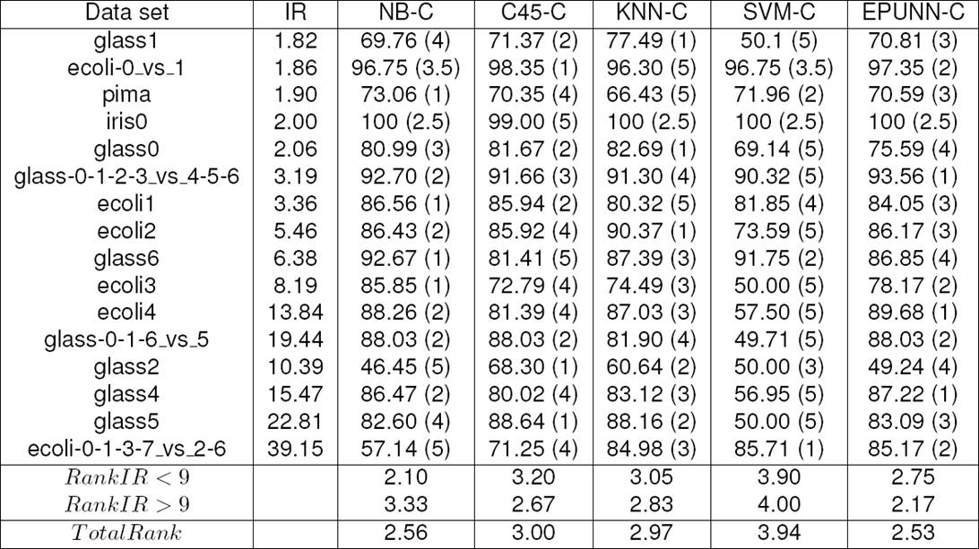
According to the results obtained, see Table 7, we statistically analyzed the results to detect significant differences in the AUC of the obtained models by the different learning methods. The multi-comparison Friedman’s test rejected the null hypotheses that all the systems performed the same on average with p = 0.0824. The obtained pvalue > 0.05 shows that there does not exist a significant difference between the five algorithms under study on the imbalanced data sets. However, we can note a tendency to robustness of the EPUNN classifier with the increment of the imbalanced level. To validate these results, we also applied the Holm’s step-up and step-down procedure sequentially to test the hypotheses ordered by their significance. As it can be observed in Table 8, the Holm’s test at α = 0.05 detected a significant difference between EPUNN and SVM-C, this is an important difference with respect to the exper/iment #1. Furthermore, in experiment #3, the winner algorithm was EPUNN.
4.4.4 Experiment #4
In the fourth experiment we evaluated the performance of the EPUNN classifier with the test accuracy metric. We used a ten-fold cross validation procedure with 5 different random seeds over each data set. The average values of the results for each collection are shown in Table 9. The last row shows the average rank of EPUNN over each data sets group.
Table 9 Accuracy of EPUNN on classical data sets and EPUNN on data sets with missing values
| % Missing | Data set | EPUNNvsMV | EPUNNvsNotMV | Data set | Difference |
| 70.58 | australian+mv | 77.97 | 86.67 | australian | deteriorate |
| 48.21 | ecoli+mv | 81.85 | 76.82 | ecoli | progress |
| 32.67 | iris+mv | 94.00 | 96.00 | iris | deteriorate |
| 50.65 | pima+mv | 75.01 | 76.71 | pima | deteriorate |
| 70.22 | wine+mv | 88.76 | 96.01 | wine | deteriorate |
| 28.83 | automobile-mv | 53.10 | 58.38 | automobile | deteriorate |
| 32.28 | bands-mv | 67.27 | 69.24 | bands | deteriorate |
| 3.15 | breast-mv | 71.49 | 72.93 | breast | deteriorate |
| 48.39 | hepatitis-mv | 80.32 | 80.36 | hepatitis | deteriorate |
| 2.29 | wisconsin-mv | 96.23 | 96.36 | wisconsin | deteriorate |
| Rank | 1.9000 | 1.1000 |
According to the results obtained, see Table 9, we statistically analyzed the results to detect significant differences. We used the accuracy metric in EPUNN over classical data sets (EPUNNvsNotMV) and in EPUNN over missing values data sets (EPUNNvsMV). The multi-comparison Friedman’s test rejected the null hypothesis that both cases (with and without missing values) behaved equally with a p = 0.0114. The obtained pvalue < 0.05 shows that there exists a significant difference. To check this results, we also applied the Holm’s step-up and step-down procedure sequentially to test the hypotheses ordered by their significance. As it can be observed in Table 10, Holm’s test at α = 0/.05 showed significant differences between EPUNNvsNotMV and EPUNNvsMV.
Table 10 Holm / Hochberg Table for α = 0.05
| i | algorithm | z = (R 0 - Ri )/SE | p | Holm/Hochberg/Hommel |
| 1 | EPUNNvsMV | 2.5298 | 0.0114 | 0.0500 |
Based on these results, we can conclude that the EPUNN algorithm was able to handle missing data, but in this kind of data, a significant performance deterioration was manifested.
5 Conclusions and Future Work
In this paper, we tested the competitiveness of an EPUNN algorithm for classification task, generally using accuracy as the evaluation metric. Furthermore, AUC metric was used in evaluation of imbalanced data sets. As a result of the four experiments described in section 4.4, we can make the following conclusions:
- From experiment #1 described in subsection 4.4.1, we conclude that there does not exist a significant difference between EPUNN and the four algorithms assessed. We based this statement on the evaluation done over 21 benchmark data sets. For this reason, we recommend its use for the classification task.
- From experiment #2 described in subsection 4.4.2, we determined experimentally that the accuracy of EPUNN rapidly worsen in the presence of noise. For that reason, we do not recommend its utilization in noisy environments.
- From experiment #3 described in subsection 4.4.3, we can note a tendency to robustness in EPUNN despite of the growth of the imbalance ratio.
- From experiment #4 described in subsection 4.4.4, we can conclude that EPUNN is able to handle missing data; but in this kind of data, a significant performance deterioration was manifested.
In future work, we can also assess the impact of irrelevant attributes on the performance of EPUNN and the influence of noise using other data sets. Also, we can use more different kinds of data sets with missing values, since the nature of values and their distribution affect the performance of the classifiers

