nueva página del texto (beta)
 Inglés (pdf)
 Artículo en XML
 Referencias del artículo
 Enviar artículo por email
 Citado por SciELO
  Similares en
SciELO
Similares en
SciELO 
 Permalink
1 Introduction
A constrained optimization problem is usually written as a non-linear programming problem (NLP) 34 of the following form:
In the above NLP problem, the function f is the objective function, where
f(X) : RD →
R there are D variables, X =
(x1,.., xD) is a vector
of size D, X ∈ RD , where
RD represents the entire search space,
gi are the inequality constraints,
hj are the equality constraints, and
The equality constraints can be transformed into the inequality form, and then, they can be combined with the other inequality constraints as follows:
Thus, the optimization goal is to find a feasible vector X to minimize the objective function.
When the vector X contains a subset of μ and ν vectors of continuous real variables and integer variables, respectively, |μ| + |ν| = |x| = D, the NLP problem becomes a mixed-integer nonlinear programming problem (MINLP).
Non-convex NLPs and MINLPs are commonly found in real-world situations. Therefore, the scientific community continues to develop new approaches for obtaining optimal solutions with acceptable computational time in various engineering and industrial fields. For example, in design optimization, the design objective could be simply to minimize the cost or maximize the efficiency of production; on the other hand, the objective could be more complex, e.g., controlling the highly non-linear behavior of pH neutralization processes in a chemical plant. The need to solve practical NLP/MINLP problems has led to the development of a large number of heuristics and metaheuristics over the last two decades 27,33,36. Metaheuristics, which are emerging as effective alternatives for solving NP-hard optimization problems, are strategies for designing or improving very general heuristic procedures with high performance in order to find (near-)optimal solutions; the goal is efficient exploration (diversification) and exploitation (intensification) of the search space. For example, we can take advantage of the search experience to guide search engines by applying learning strategies or incorporating probabilistic decisions.
Strategies such as differential evolution (DE), ant and bee algorithms, particle swarm optimization (PSO), and cuckoo search have been effectively applied to many research areas, including process design 2,3. Nevertheless, these approaches have a drawback in that they require the setting of several parameters and components, e.g., population size, number of generations, recombination probability, mutation operator, and selection function, as well as the handling of constraints. Therefore, selecting the best combination of these parameters/components leads to complexity of the metaheuristic algorithms. In other words, the various possible combinations of the parameters drastically affect the performance of the algorithms.
Nowadays, methodologies such as hyper-heuristics minimize human interference in the tuning and design of heuristics or metaheuristics adapted for solving a problem in a particular domain 3. In this paper, an approach for solving non-convex MINLP problems is presented. Our analysis is based on a DE hyper-heuristic methodology, which is able to choose from among 18 DE models for low-level heuristics and tune the most important parameters through a self-adaptation mechanism.
The remainder of this paper is organized as follows. Section 2 describes the DE algorithm. Section 3 outlines the hyper-heuristic algorithm. Section 4 reviews some related studies. Section 5 describes the proposed approach. Section 6 presents an illustrative example to show how a population evolves through generations before reaching the global optimum. Section 7 describes a set of problems on process synthesis and design for an experimental setup to show the applicability and efficiency of our approach in the case of non-convex MINLP problems. Section 8 presents the corresponding results. Finally, Section 9 summarizes our findings and concludes the paper with a brief discussion on the scope for future work.
2 Differential Evolution (DE) Algorithm
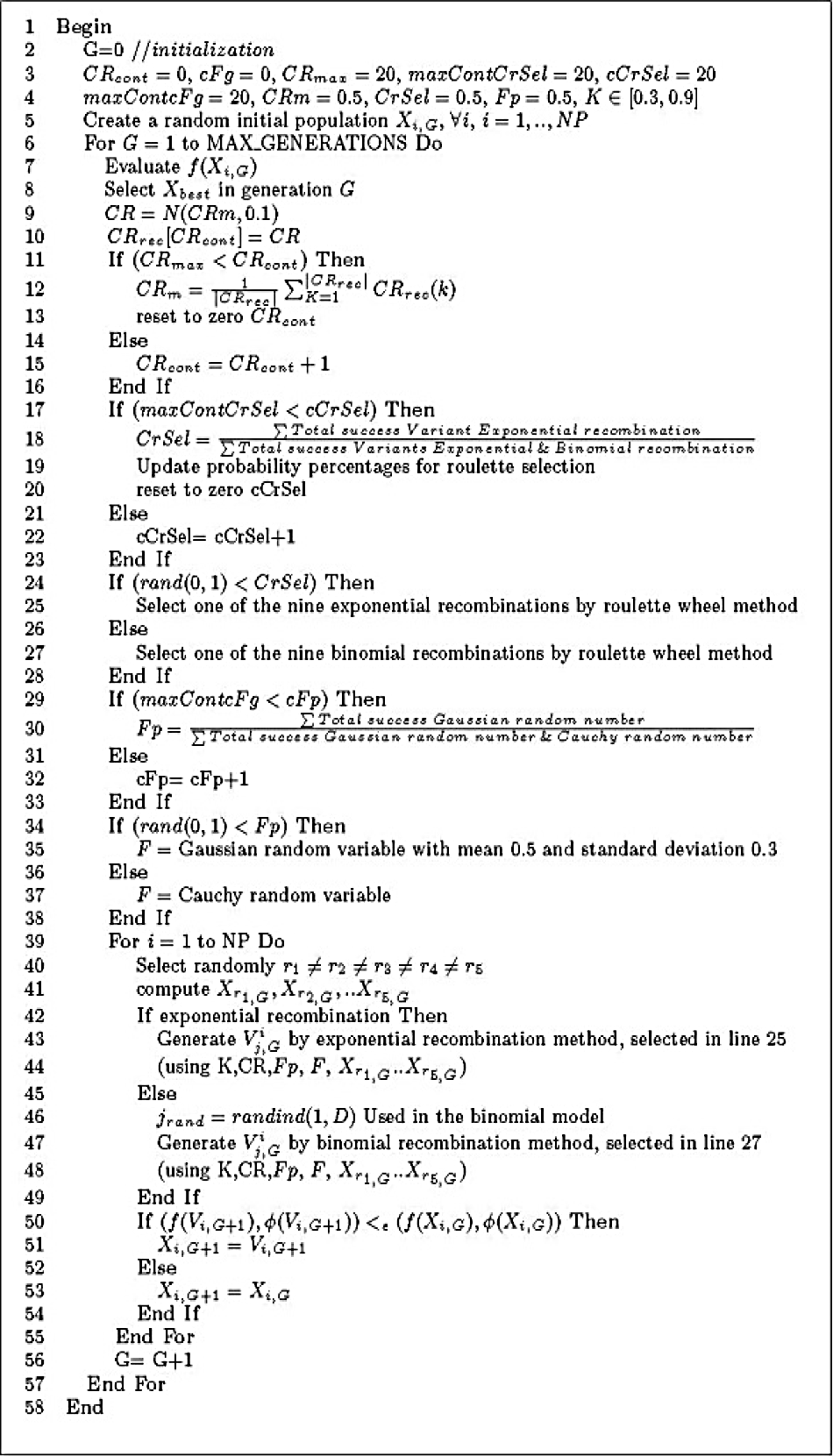
Since its implementation in 1995 by Storn and Price 37,38, DE has gained wide acceptance because it is particularly easy to work with, having only a few control variables that remain fixed throughout the entire optimization procedure. DE is a search method that uses a set of vectors xi,G as the population in each generation. The algorithm starts from a randomly generated initial population until a satisfactory one is obtained. The population size does not change during the evolutionary process; thus, the algorithm is a population-based stochastic search technique classified as floatingpoint encoded. A DE pseudo-code is shown in Figure 1.

The main concept underlying DE is a new schema to generate vectors. The mechanism is as follows. A new vector is generated by adding the weighted difference between two member vectors of the population to a third member (see Figure 1 and focus on line 11).
Both vectors, i.e., the newly generated vector and the original vector, are rated by an evaluation method. The vector with the best fitness is chosen, and it replaces the losing vector in this comparison (see Figure 1: the If statement in line 16 and the corresponding Else starting in line 18). There are several variants of the mutation scheme of DE. The notation used in the literature is DE / φ / φ / ψ, where φ denotes the base vector to be disturbed, i.e., the mechanism for constructing the mutant vector, φ denotes the number of pairs of vectors to be disturbed, and ψ denotes the crossover type (exp: exponential; bin: binomial). Several DE schemes are presented in Appendix A.
Line 11 contains the mutation operator, where r1 ≠ r2 ≠ r3 are randomly generated vectors ∈ [1,NP] and NP is the population size. F is a scaling factor that typically ∈ (0,1]; it controls the amplification of the difference vector. Lines 10 to 14 contain the crossover operator, which is represented by the If - Else statement, where the crossover constant is denoted by CR ∈ [0,1] and jjrand is a randomly chosen index ∈ {1,2,..,D}; D is the number of variables in the problem. CR and F are user-defined parameters. CR is highly sensitive to the property and complexity of the problem, while F is related to the convergence speed. The DE model described above is known as DE/rand/1/bin, where rand denotes the base vector to be disturbed, 1 denotes the number of pairs of vectors to be disturbed, and bin denotes the recombination adopted.
3 Hyper-Heuristics
A hyper-heuristic is a search method or learning mechanism for selecting or generating simpler heuristics to solve computational search problems. The hyper-heuristic framework consists of two main parts: a high-level methodology and a number of low-level heuristics. Given a particular problem instance or class of instances, the high-level method provides the means to exploit the strength of multiple low-level heuristics, where each heuristic can be useful at different stages of the search. The solution is either accepted or rejected based on an acceptance criterion. The heuristic selection and acceptance methods are the most important components of a hyper-heuristic. The main feature of the hyper-heuristic approach is that the high-level heuristic performs a search over the space of the low-level heuristics rather than a direct solution space. A domain barrier between the levels prevents any problem-specific information from being passed to the hyper-heuristic level, thereby allowing for selection from among the low-level heuristics without the need for domain knowledge. The development of hyper-heuristics is mainly motivated by the need for algorithms that are more generally applicable than most current implementations of search methods. The low-level heuristics can be designed in advance or created simultaneously during runtime from a set of potential components. Thus, the hyper-heuristic approach aims to reuse the heuristics over unseen instances and raise the level of generality at which an optimization system can operate.
In the hyper-heuristic framework, the high-level heuristic has no knowledge of the problem-domain concealed in the low-level one. In turn, the low-level heuristic is not aware of the learning mechanism used to choose its heuristic (DE models) in the high level. This process introduces the concept of plug-and-play of heuristics (DE models).
In recent years, hyper-heuristics have been employed in several applications such as the bin packing problem 29, 2D strip packing 8, production scheduling 30, constraint satisfaction problems 28, and the vehicle routing problem 25. In addition, some hyper-heuristics use a metaheuristic as a high-level methodology or mechanism to select or generate low-level heuristics, with effective and encouraging results. A survey of hyper-heuristics can be found in 7.
4 Related Work
In the existing literature, it is possible to find several DE-based approaches for solving constrained optimization problems.
In 23, Lampinen proposed an extension of DE. The method consists of a modification to the selection operator with a new selection criterion for handling the constraint functions. The selection is based on Pareto dominance in the effective constraint function space, and the approach does not introduce any extra search parameters to be set by the user. A DE/rand/1/bin strategy was used.
In 21, a penalty function is designed to handle the constraints and a co-evolution model is incorporated into a DE algorithm to perform evolutionary search in spaces of solutions and penalty factors. Both evolve interactively and self-adaptively; thus, a satisfactory solution and suitable penalty factors can be obtained simultaneously. A DE/best-rand/1/bin strategy was used.
The aim of the approach proposed by Mezura et al. in 26 is to increase the probability that each parent generate a better offspring by allowing each generation to generate more than one offspring using a different mutation operator that uses information of the best solution and the current parent to find new search directions. A DE/rand/1/bin strategy was used.
In 24, Mallipeddi et al. showed how a compendium of constraint-handling techniques used with evolutionary algorithms can be effectively applied to differential evolution. These include the superiority of feasible solutions, self-adaptive penalty, Ԑ-constraint, and stochastic ranking. The authors showed that the effectiveness of conventional DE in solving a numerical optimization problem depends on the selected mutation strategy and its associated parameter values. Thus, different optimization problems require different mutation strategies with different parameter values. The DE/rand/2/bin and DE/current-to-rand/1/bin strategies were used.
A DE variant considered as a state-of-the-art algorithm, namely, SaDE 32, incorporates a learning strategy in the mutation phase, which probabilistically selects one out of two available learning strategies, DE/rand/1/bin or DE/current-to-best/2/bin, and applies it to the current population. Furthermore, the control parameter CR is self-adapted based on the previous learning experience, and a quasi-Newton method is used as a local search method.
In 31, the SaDE algorithm was compared with several parameter-adaptive DE variants. It was found that the SaDE algorithm could evolve suitable strategies and parameter values as the evolution progressed and that the learning period parameter had an insignificant impact on the performance. In addition, the algorithm was more effective in obtaining high-quality solutions over a suite of 26 bound-constrained numerical optimization problems.
In 20, the original search method in the SaDE algorithm was substituted by a sequential quadratic programming method.
A comparison between a neighborhood search strategy and the SADE algorithm can be found in 45. This strategy affects the F parameter, which is related to the convergence speed. Thus, it is effective in escaping from local optima when searching environments without prior knowledge about what kind of search step size is preferred. A hybridization of SaDE with the neighborhood search algorithm led to the following approach: the neighborhood search strategy, the learning strategy in the mutation phase, and three self-adaptive mechanisms for the three parameters, namely, the scale factor F, the crossover rate CR, and the mutation strategy. The authors reported that such a hybridization is significantly superior to both neighborhood search algorithm and SaDE individually.
In 4, a self-adaptive mechanism for changing two DE control parameters, F and CR, during the optimization process with a small and varying population size was presented. A DE/rand/1/bin strategy was used.
In 42, a success-history-based adaptive DE was proposed. The strategy uses historical memory in order to adapt the control parameters F and CR.
The use of eigenvectors of the covariance matrix of individual solutions, which makes the crossover rotationally invariant in DE, was proposed by Guo et.al in 18. The incorporation of eigenvector-based crossover in six state-of-the art DE variants showed either solid performance gains or statistically identical behavior. The concept of opposition-based learning has been applied to improve the performance of metaheuristic algorithms and machine-learning algorithms. The method tries to find a better candidate solution by simultaneously considering an estimate point and its corresponding opposite estimate.

In 19, a partial opposition-based learning methodology was applied to an adaptive DE algorithm.
In 6, an adaptive DE based on competition among several strategies was used. The approach uses a rotation-invariant current-to-best mutation in the algorithm. The aim is to increase the efficiency of DE on rotated or composite functions.
In 43, a hyper-heuristic based on DE was proposed. The approach consists of two phases. The first phase is responsible for selecting the type of recombination to be adopted (either bin or exp). At the beginning of the search process, a training stage based on the maximum number of generations and a random descent selection mechanism is required to initialize the expected values for each of the DE variants. The second phase is responsible for selecting the specific model to be applied for generating the next generation. Random selection and roulette wheel selection mechanisms are used. Stochastic ranking is incorporated for handling the constraints. Twelve crossover model strategies are used as low-level heuristics in the hyper-heuristic framework.
Further details about recent research on hyper-heuristics based on DE can be found in 16.
In spite of the above-mentioned efforts, there remains a considerable scope for improving DE performance, e.g., by using strategies or proposing new strategies of self-adaptation for parameter control, mutation, or constraint handling, or by applying learning mechanisms that have not been used previously in DE frameworks.
5 Proposed Approach
The motivation of our approach is to solve non-convex MINLP problems with applications in process design by using a DE-based hyper-heuristic algorithm. Our framework includes self-adaptive parameters, an Ԑ-constrained method for handling constraints, 9 mutation model strategies, and a binomial and exponential crossover model; the combination mutation-crossover allows to have a maximum of 18 Differential Evolution models. The overall flow of our approach is shown in Figure 2 and the pseudo-code is shown in Figure 3.

Our framework includes the strategies described in subsections 5.1 to 5.5.
5.1 Self-Adaptive Parameters
The use of the DE self-adaptive mechanism to make a DE solver more robust and efficient is reported in 5; in addition, its advantages and disadvantages are discussed there.
Our self-adaptation scheme focuses on the three main components of the DE algorithm that directly affect the performance and the quality of the solution, namely, the mutation, the crossover, and the scale factor F. Lines 9 to 15 in Figure 1 show the use of these components without a self-adaptation mechanism. In order to achieve autotuning of these parameters, a learning period was incorporated. The basic idea is to define a specified number of generations to collect data and a counter of iterations. When the counter exceeds the number of generations proposed, it will be reset once the variable is updated with a new value.
5.2 Self-Adaptation of Crossover Rate CR
Our crossover strategy is based on SaDE 32,45, where the CRm variable is set to 0.5 initially; after a determined number of generations, CRm will be updated according to equation 3. Thus, CRm is used as the mean value in the Gaussian function given by equation 4 in order to compute the crossover rate (CR) that will be used in the recombination method:
 (3)
(3)
The proposed crossover includes a strategy of selection to choose between a binomial or exponential method, in contrast to the SaDE algorithm that only uses binomial crossover.
5.3 Self-Adaptation of the Scale Factor F
Because the scale factor F is related to the convergence speed, its self-adaptation strategy incorporates a move-generation mechanism as a neighborhood search operator in the DE algorithm. This can be observed in 45, 46, where the scale factor F is replaced by equation 5:
 (5)
(5)
where Ni (0.5,0.3) denotes a Gaussian random number with mean 0.5 and standard deviation 0.3, and ∂i . denotes a Cauchy random variable with scale parameter t = 1. In our approach, Fp in equation 5 will be self-adapted according to equation 6:
where TSGRN denotes the success Gaussian random number and CRN is the success Cauchy random number.
5.4 Self-Adaptation of Mutation Strategies
The impact of the various DE search operators on the exploration/exploitation of the search space is not the same. Certain mutation operators are more oriented toward exploitation, e.g., DE/best/1, whereas others are more oriented toward exploration, e.g., DE/rand/1 13. Thus, it can be difficult to choose the most efficient mutation operator, and a problem-dependent parameter may affect the performance of the algorithm. A determined combination of DE parameters can be suitable for one problem but unsuitable for another 44. In order to raise the level of generality, our approach incorporates in the hyper-heuristic framework a selection method for choosing the type of recombination to be applied for generating the next population, either exponential or binomial, by a random process. The method includes a variable, CrSel, which is set to 0.5 initially; after a determined number of generations, CrSel will be self-adapted according to equation 7 (see Figure 3: lines 17 to 23).
This set of heuristics consists of nine promising mutation strategies reported in the literature, each for the binomial and exponential models; a roulette wheel method is used to choose the mutation variant to be adopted, see Figure 4.
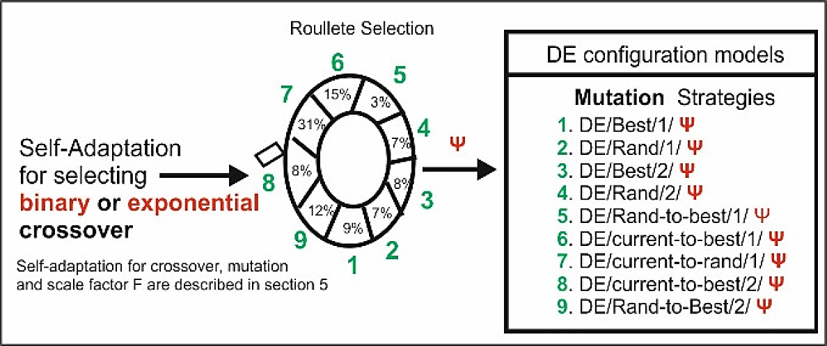
The maximum number of possible crossover-mutation combinations are 18. These 18 DEmodels are used as low-level heuristics shown in Appendix B. For example, if the type of recombination selected is exponential, the roulette wheel method will choose from among the nine mutation strategies for exponential recombination, starting with a probability of 1/9 for each strategy to be selected; the probabilities will be updated when CrSel is updated (see line 19 in Figure 3). The complete mutation strategies used in our approach are presented in Appendix B.
where TSVER denotes the success variant exponential recombination and BR is the success binomial recombination.
5.5 Constraint Handling
The Ԑ-constrained method was proposed by Takahama 40. It is based on the definition of a constraint violation φ(x) that is obtained from equation 8 or equation 9, which are adopted as a penalty in penalty function methods.
where p ∈ Z+ and φ(x) is the maximum of all constraints or the sum of all constraints. Thus, φ(x) indicates by how much a search point x violates the constraints and the membership in the feasible region F. Feasible solutions exist in S, where F ⊆ S and S is the search space. The values of φ(x) that can be obtained are given by equation 10.
An order relation on the set (f (x), φ(x)) is known as an Ԑ level comparison and defined by a lexicographic order in which φ(x) precedes f(x), favoring the feasibility of x over the minimization of f(x). The comparisons are made according to the rules given by equations 11 and 12:
 (11)
(11)
 (12)
(12)
The opposite cases where ԑ = 0(<0 and <0) and ԑ = ∞(<∞ and ≤∞) are equivalent to the lexicographic order in which the constraint violation φ(x) precedes the function value f(x) on the one hand and to the ordinal comparison < and ≤ between function values on the other hand, respectively. In order to obtain high-quality solutions, the Ԑ level is statically controlled by equation 13. It is updated until the generation counter k reaches the control generation Tc . When the generation counter exceeds Tc , the Ԑ level is reset to zero in order to obtain solutions without constraint violation. Note that cp is a user-defined parameter for controlling the reduction speed of the Ԑ tolerance.
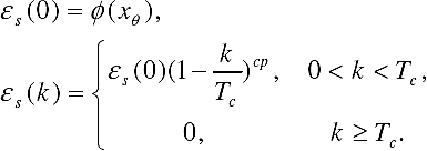 (13)
(13)
The Ԑ-constrained method with static control was incorporated into our approach. We assume that p=1 in equation 9 for a simple sum of constraints.
For the function evaluation, in order to handle integer variables, real values are converted into integer values by truncation. The handling of binary variables is given by equation 14.
where xi is a continuous variable, 0 ≤ xi ≤1. For the boundary constraint, the same handling mechanism that is used for continuous variables is applied (0 is assigned to the lower bound and 1 is assigned to the upper bound).
5.6 Our Approach versus SaDe: A Comparison between Designs
The SaDE algorithm uses only a binomial crossover operator and 2 mutation strategies selected by a random process 32. In the last version, it incorporates 4 mutation strategies selected by the roulette method improving the performance 20.
The comparative analysis of binomial and exponential crossover variants provides information about the influence of the crossover parameter on the behavior of DE. The dependence between the mutation probability and the crossover parameter is linear in the binomial case and nonlinear in the exponential one. The use of both types of crossover together makes the algorithms more robust 49. Nevertheless, it is not possible to generalize, since a combination of parameters can be effective for a problem or instance of one problem and ineffective for another. In order to combat these weaknesses, our approach encapsulates a set of predefined heuristics (DE models as low-level heuristic) for the given problem, a fitness evaluation function, and a specific search space. The high-level heuristic decides which low-level heuristic (DE model) will be chosen. This can be achieved with a learning mechanism that evaluates the quality of the heuristic (DE model) solutions, so that they can become general enough to solve unseen instances of a given problem. In the hyper-heuristic framework, it is possible to add or remove low-level heuristics without the need to code the entire algorithm again. The main design differences between SaDE and our approach are presented in Table 6 (Illustrative example).
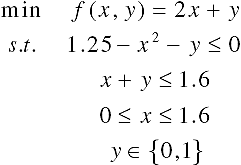
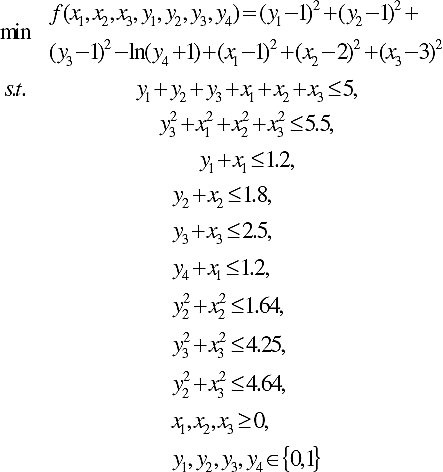
Consider the following quadratically constrained linear program taken from 34:
where the global optimum reported in the literature is x=(-1.414214, -1.414214) with f= -2.828427. Two local solutions are at x=(-1,0) with f= -1 and x=(1,0) with f=1. Thus, the solution is required to be in the region bounded by all the constraints. Figure 5 shows how this problem is solved by applying the proposed approach.
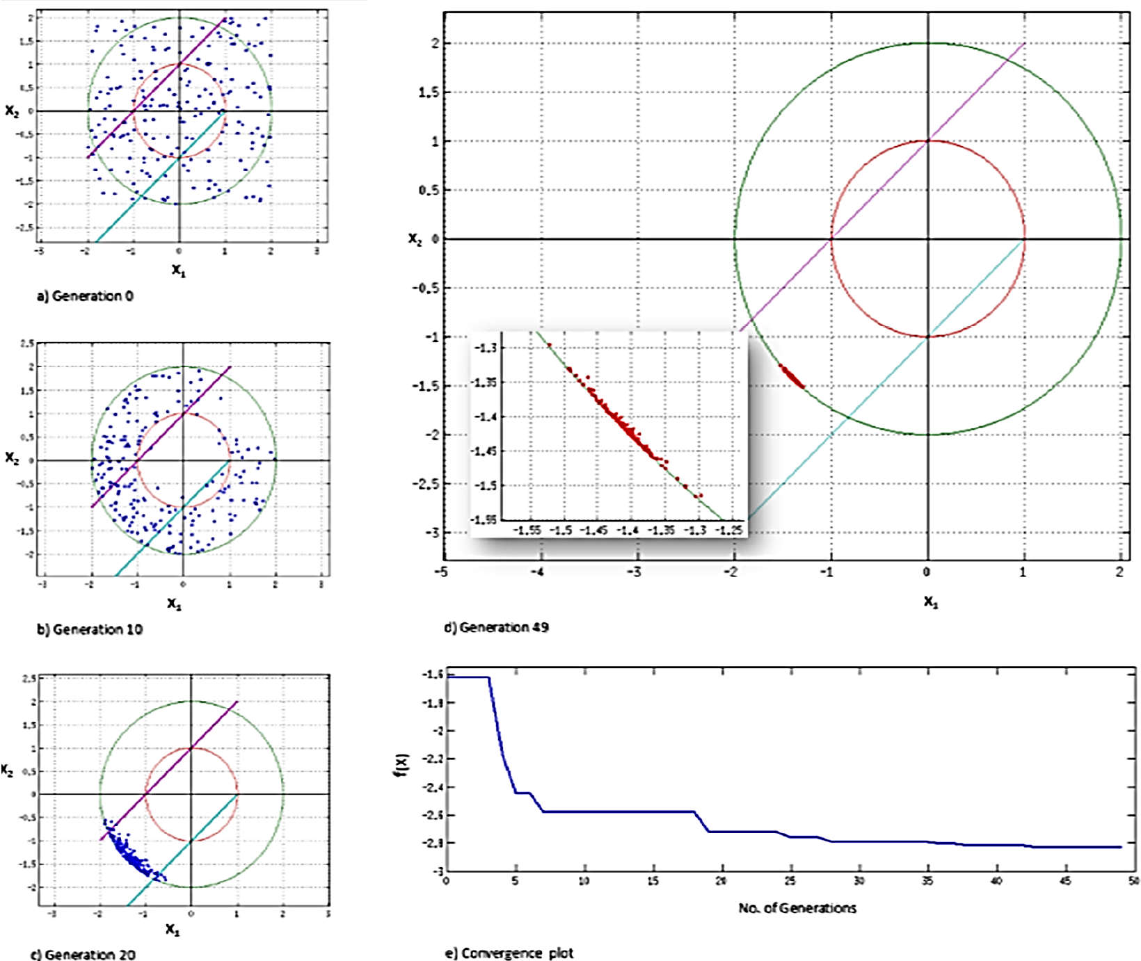
Fig. 5 Evolution of the population from the initial generation (a) to the end generation (d) and the full trace of the convergence plot (e)
In order to have sufficient data and show their behavior, the parameters used are the population size Np = 200 and the maximum number of generations MaxGen=50; each of the self-adaptive variables, namely, CRsel, fp, and CRm, starts with a value of 0.5. After 20, 20, and 5 generations, respectively, the variables are updated ("learning period"). The algorithm was able to find the global optimum in 0.018 s, with 10200 evaluations of the objective function.
In an experimental test with a population size of Np = 25 and the maximum number of generations MaxGen=30, the global optimum was found in 0.00343 s, with 775 evaluations of the objective function.
7 Case Studies
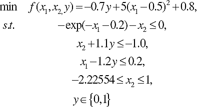
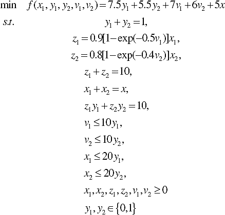
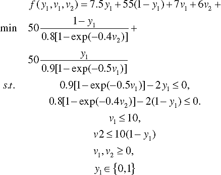
Seven problems from the field of chemical engineering, which involves complex non-convex optimization problems with continuous and discrete variables, were considered in the present study. Definitions of these Benchmark Problems are presented in Appendix A.
8 Results
Our approach, namely, the DE-HH algorithm, is implemented in C and compiled using GCC version 4.8.2. All computations were carried out on a standard PC (Linux Kubuntu 14.04 LTS, Intel core i5, 2.20 GHz, 4 GB).
The reliability and efficiency of our approach were compared with those of several state-of-the-art algorithms reported in the literature. The comparison involves the mean values of ten experiments for each problem; it includes two parts as follows.
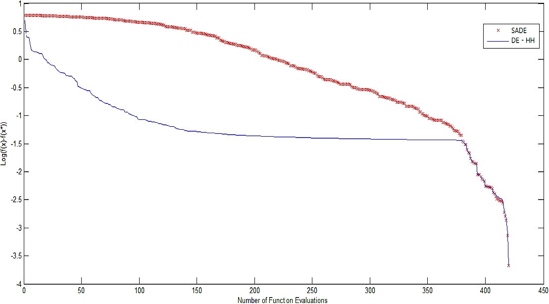
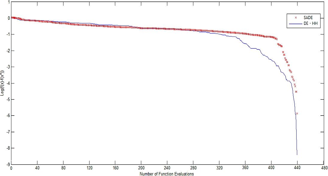
In the first part, a comparison is made against the SaDE algorithm 20 measuring convergence speed and quality of results. The results are based on the best, the worst, mean, and standard deviation; these are listed in Table 2. A convergence graph for each problem was plotted. The graph shows the median run of the total runs with termination by the max number of function evaluations obtained. We use the function value of the problem without penalties, f(x), and the fitness value of best-known solution, f(x*). In the log graphs, the x-axis corresponds to the number of function evaluations and the y-axis corresponds to the log (f(x)-f(x*)), see Figures 6 to 12 (7, 8, 9, 10, 11).
Table 2 Comparison between DE-HH and SADE algorithm
| SADE | DE-HH | ||||||||
|---|---|---|---|---|---|---|---|---|---|
| Problem | Best Reported | Best | Worst | Mean | Std. | Best | Worst | Mean | Std. |
| 1 | 2.0000 | 2.0000 | 1.8269 | 1.9711 | 5.91E-02 | 2.0000 | 1.9237 | 1.9865 | 2.63E-02 |
| 2 | 2.1240 | 2.1236 | 2.0786 | 2.1093 | 1.91E-02 | 2.1240 | 2.0936 | 2.1171 | 1.06E-02 |
| 3 | 1.0765 | 1.0693 | 1.0438 | 1.0695 | 1.02E-02 | 1.0762 | 1.0534 | 1.0719 | 6.98E-03 |
| 4 | 99.2452 | 99.2450 | 99.1184 | 99.2202 | 4.14E-02 | 99.2451 | 99.1963 | 99.2318 | 1.83E-02 |
| 5 | 3.5574 | 3.5461 | 3.0530 | 3.4649 | 1.52E-01 | 3.5574 | 3.4384 | 3.5294 | 3.62E-02 |
| 6 | 32217.4 | 32216.96 57 | 32214.96 18 | 32216.14 82 | 6.50E-01 | 32217.43 50 | 32215.36 81 | 32216.6453 | 8.52E-01 |
| 7 | 38499.8 | 38498.21 7 | 38495.32 8 | 38497.03 | 1.33E+00 | 38499.76 19 | 38496.53 2 | 38498.9411 | 1.29E+00 |
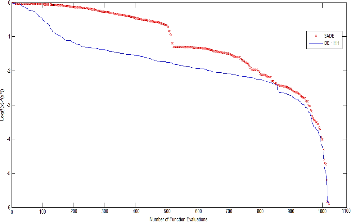


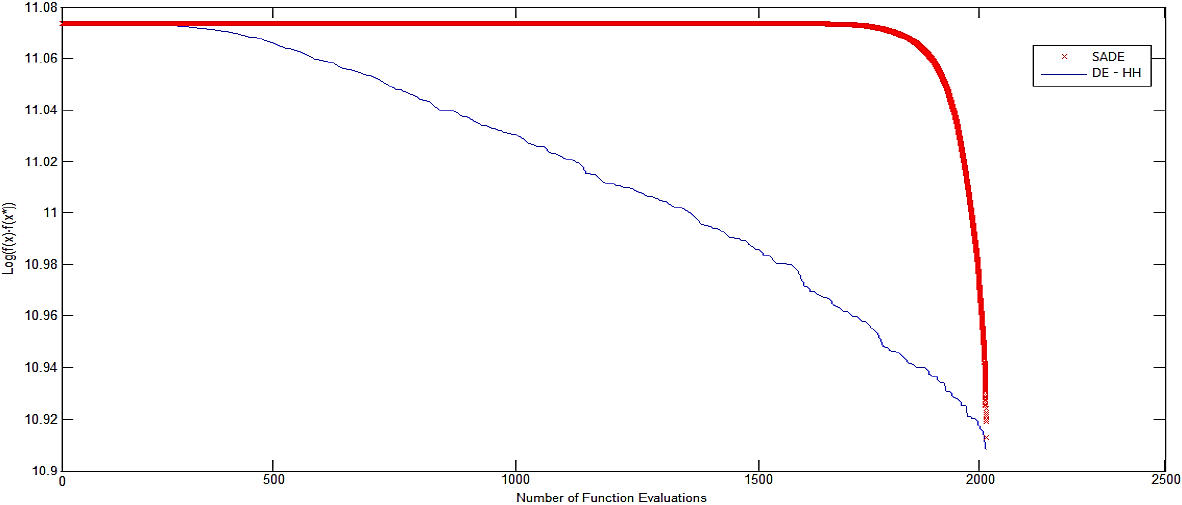
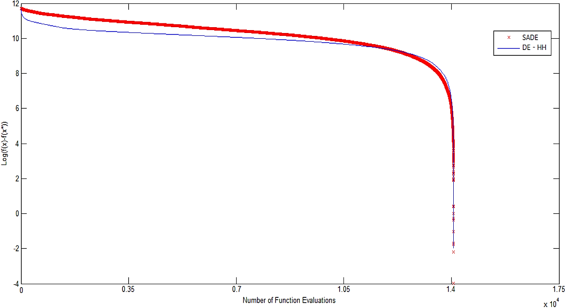
The comparison shows that our approach improves the best results reported of the SaDE algorithm, including better mean and standard deviation.
In the second part, a comparison is made against genetic algorithm (GA), simplex-simulated annealing (M-SIMPSA & M-SIMPSA-pen variant), evolution strategies (ES), and modified differential evolution (MDE); all these algorithms are reported in 1, while particle swarm optimization (R-PSO_c) is reported in 47.
The results are based on the percentage of convergences to the global optimum (NRC) and the average number of objective function evaluations (NFE); these are listed in Table 3, where the CPU time in seconds is also reported. The best results obtained are listed in Table 4. For Problem 1, a comparison shows that the NFE for DE-HH is around 30.82\% less than that for M-SIMPSA and 93.82\% less than that for GA.
Table 3 DE-HH Results
| Problem | NFE | NRC | CPU-Time |
|---|---|---|---|
| 1 | 420 | 100 | 0.002111 |
| 2* | 440 | 100 | 0.002169 |
| 3 | 1020 | 100 | 0.007012 |
| 4* | 1680 | 100 | 0.012646 |
| 5 | 6030 | 100 | 0.047243 |
| 6 | 2020 | 100 | 0.026431 |
| 7 | 14600 | 100 | 3.841227 |
Table 4 Percent reduction in NFE due to DE-HH as compared with the best algorithm reported
| Problem No. | Our approach | % Reduction in NFE by DE-HH | Best algorithm reported |
|---|---|---|---|
| 1 | 30.81 % | M-SIMPSA | |
| 2* | 10.20% | MDE | |
| 3 | 41.68% | ES | |
| 4* | DE-HH | 6.51% | MDE |
| 5 | 10.14% | ES | |
| 6 | 20.35% | ES | |
| 7 | 2.67% | R_PSO_C |
Our approach improves the NFE and NRC of the M-SIMPSA reported as the best for this problem.
For Problem 2, the NFE for DE-HH is 97.3% less than that for GA. Moreover, for Problems 1 to 7, the NFE for DE-HH is around 40.42%, 10.20%, 48.33%, 6.51%, 49.38%, 63.23%, and 64% less, respectively, than that for MDE. For Problem 7, our approach improves the NFE and NRC of the R_PSO_c algorithm, which has been reported as the best. A summarized comparison of DE-HH with the best algorithms reported for each problem is presented in Table 5.
Table 5 Comparison of DE-HH, GA, M-SIMPSA, M-SIMPSA-pen, ES, MDE & R-PSO_c
| ratio NFE/NRC | |||||||
| Problem no. | GA | M- SIMPSA | M-SIMPSA- Pen | ES | MDE | R-PSO_c | DE-HH |
| 1 | 67.87 | 6.13 | 162.82 | 15.18 | 7.05 | -- | 4.20 |
| 2* | 139.39 | 127.49 | 144.40 | 22.55 | 4.90 | 35.00 | 4.40 |
| 3 | 1070.46 | #/0 | 380.42 | 17.49 | 19.74 | -- | 10.20 |
| 4* | 224.89 | 147.38 | 422.95 | **/0 | 17.97 | 40.00 | 16.80 |
| 5 | 1712.96 | 371.816 | 657.22 | 67.10 | 119.14 | 300.00 | 60.30 |
| 6 | 371.67 | 315.057 | 357.43 | 25.36 | 54.95 | -- | 20.20 |
| 7 | α | #/0 | 2799.33 | **/0 | 405.50 | 166.66 | 146.00 |
#Executionn halted,
**Converged to a non-optimal solution,
--such results were not available for the corresponding algorithm
α: 225176 of NFE and zero of NRC reported
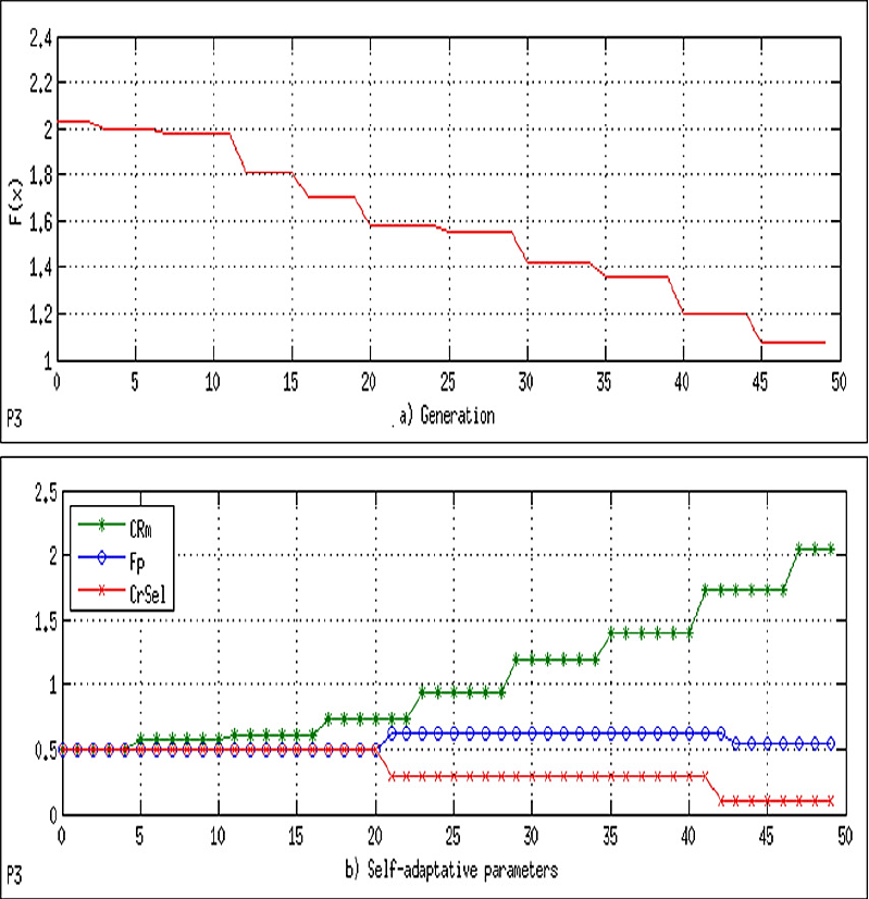
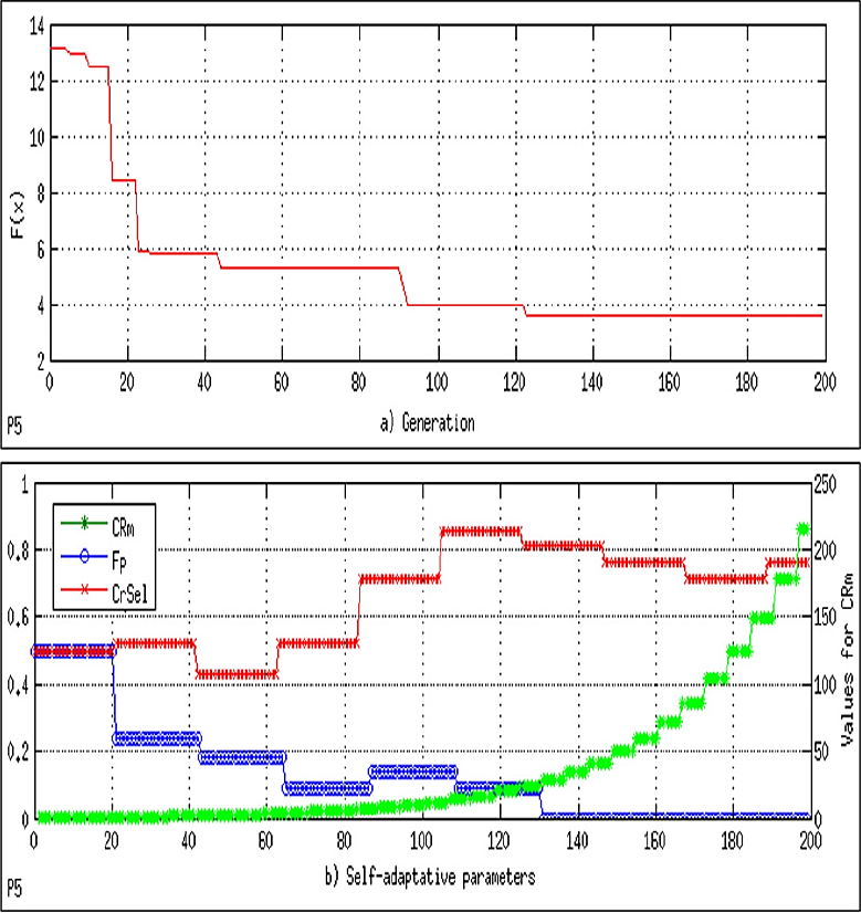
The convergence plot, labeled as (a), and the behavior of the self-adaptive parameters (CRm, Fp, and CrSel), labeled as (b), for each problem are shown in Figures 4 to 10.
For the convergence plot, the x-axis corresponds to the number of generations and the y-axis corresponds to the values of f(x). For the self-adaptive parameters, the x-axis corresponds to the number of generations and the y-axis corresponds to the obtained values of CRm, Fp, and CrSel. Observe that in Figures 5 to 7, the y-axis appears with different scales on the left and right sides. More specifically, the y-axis on the left corresponds to Fp and CrSel, and the y-axis on the right corresponds to CRm. CPU time in seconds.


9 Conclusions
This paper proposed a differential-evolution-based hyper-heuristic (DE-HH) approach for the optimization of mixed-integer non-linear programming (MINLP) problems. Self-adaptive mechanisms of the control parameters in the DE algorithm are carried out over the hyper-heuristic framework. The constraints are handled by the epsilon-constrained method. The choice functions of the proposed framework can adaptively select appropriate low-level heuristics from a set of 18 DE variants. Additional mutation strategies and different crossover schemes can also be applied to the hyper-heuristic framework in order to adapt it to a particular problem.
We conducted experimental studies on test instances of process synthesis and design that represent difficult non-convex optimization problems often encountered in the field of chemical engineering. The results, which were based on the percentage of convergences to the global optimum (NRC) and the average number of objective function evaluations (NFE), showed that DE-HH can find a global optimum reliably and efficiently, improving, on average, the NFE by 17.48% as compared to the best algorithms reported while maintaining the NRC at 100%. The results, which were based on the best, the worst, mean and standard deviation, showed that our approach exhibits better high quality results for all benchmark problems than SaDE algorithm, including better mean and standard deviation.
In a runtime it is possible to find DE models untouched (unused) by the hyper-heuristic. Thereby, it is unknown which of the 18 DE models are more requested for a particular problem.
Also, the contribution of each model in obtain an optimal solution, the effects of adding (or subtracting) of more DE models and its repercussions in the quality of results are unknown. Therefore, directions for future work include an analysis of sensitivity of variables and models over a hyper-heuristic environment. In addition, it is desirable to deal with larger problem instances to improve the percentage of convergences to the global optimum and improve the average number of objective function evaluations using parallelization strategies for hyper-heuristics, e.g., GPU computing and multicore resources.