New Perspectives on the Use of Spatial Filters in Magnetoencephalographic Array Processing

Zaragoza-Martínez, Claudia Carolina; Gutiérrez, David; Zaragoza-Martínez, Claudia Carolina; Gutiérrez, David

doi:10.13053/cys-20-1-2185

Services on Demand

Journal

Article

Indicators

Cited by SciELO
Access statistics

Computación y Sistemas

On-line version ISSN 2007-9737Print version ISSN 1405-5546

Comp. y Sist. vol.20 n.1 Ciudad de México Jan./Mar. 2016

https://doi.org/10.13053/cys-20-1-2185

Thematic section

New Perspectives on the Use of Spatial Filters in Magnetoencephalographic Array Processing

Claudia Carolina Zaragoza-Martínez¹

David Gutiérrez¹

^¹Centro de Investigación y de Estudios Avanzados del IPN, Unidad Monterrey, Apodaca, Nuevo León, México czaragoza@cinvestav.mx, dgtz@ieee.org

Abstract

The increase in computer power of the last few decades has allowed the resurgence of the theory behind spatial filtering (a.k.a. beamforming) and its application to array signal processing. That is the case of magnetoencephalographic (MEG) data, which relies on dense arrays of detectors in order to measure the brain activity non-invasively. In particular, spatial filters are used in MEG signal processing to estimate the magnitude and location of the current sources within the brain. This is achieved by calculating different beamformer-based indexes which usually involve a large computational complexity. Here, a new perspective on how today’s computers make it possible to handle such complexity is presented, up to the point when new and ever more complex neural activity indexes can be developed. Such is the case of indexes based on eigenspace projections and reduced-rank beamformers, whose applicability is shown in this paper for the case of using real MEG measurements and realistic models.

Keywords: Magnetoencephalography; beamformer; spatial filtering; neural activity indexes; dipole source localization

1 Introduction

The aim in spatio-temporal processing is to recover signals coming from a direction of interest, while attenuating signals from other directions. The processing element that allows such selective recovery/attenuation is known as a spatial filter or beamformer²⁶.

Although new implementations of spatial filters may improve their poor resolution when resolving signals originating from closely-located regions², they also suffer of a fundamental limitation: their performance directly depends on the number of sensing elements (aperture), independently of the number of time samples or the signal-to-noise ratio (SNR).

One might think that the limitations on aperture could be solved by using a large number of sensors (dense sensor array) and by using large-sized sensors. However, this cannot be always achieved in practice¹⁸. First, because sensors might be costly, but mainly due to the fact that adding many of them would result in an increase of computational cost. This is the result of the output of the spatial filter being a linear combination of the data acquired by M sensors at N time samples.

The computational cost increases as the number of sensors is increased, this is due to spatial filters being dependent on the covariance matrix and its inverse, which is calculated from raw data. Thus, the more sensors are considered, the greater the data matrix would be and therefore it will be more mathematically complex to calculate the covariance matrix and its inverse.

Given the limitations previously mentioned, spatial filters in biomedical applications were initially used only for interference removal, such as the case of fetal heart monitoring in²⁸. A spatial filtering method for localizing sources of brain electrical activity suited for MEG recordings was first described and analyzed in²⁷. However, their analysis only considered a sphere to model the head given the limitations in computer power at the time.

The advent of high speed digital computers nowadays has led to the emergence of many numerical techniques and with the rapidly growing computing capabilities, numerous problems of real engineering interest can now be solved with relative ease and in a much shorter time. Applying new numerical techniques in the solution of the inverse problem using a realistic model as a conductive model would result in an increased resolution, then making the estimation of the magnitude and location of a current source within the brain more accurate.

In this paper, a new perspective on how today’s computers make it possible to handle the mathematical complexity involved in MEG array signal processing is presented, up to the point when new and ever more complex neural activity analysis methods can be developed and realistic geometries to model the head can be used.

2 Methods

This section briefly reviews the concepts related to spatial filters, then the processing steps involved in their use for MEG source localization are explained.

2.1 Measurement Model

MEG is a non-invasive technique that allows the measurement of ongoing brain activity produced by the activation of multiple neurons (i.e.,50,000-100,000) in a specific area generating a measurable but extremely small magnetic field oriented at an orthogonal direction outside the head. Therefore, MEG requires an array of extremely sensitive superconducting quantum interference devices (SQUIDs) that can detect and amplify the magnetic fields generated by neurons a few centimeters away from the sensors. MEG is an attractive technology to study brain activity since magnetic fields pass unimpeded through the skull, resulting in a undistorted signature of neural activity that can be recorded at the scalp level¹³^,¹⁰.

MEG measurements are assumed to be produced by a neural source that can be modeled by an equivalent current dipole (ECD), whose magnitude is given by st=[sx(t),sy(t),sz(t)]T (assuming a Cartesian coordinate system) and located within the brain. The dipole is allowed to change in time but it remains at the same position rs during the measurements period. The ECD model holds in practice for evoked response and event-related experiments¹⁹. Then, the MEG data can be grouped, for the case of k=1,2,…,K independent experiments (trials), into a spatio-temporal matrix Yk of size M x N at the k th trial such that

Yk=[y11y12⋯y1Ny21y22⋯y2N⋮⋮⋮yM1yM2⋯yMN], (1)

where y _m(t)is the measurement at the mth sensor, for m = 1,2,…,M, and acquired at time sample t = 1,2,…,N. Under these conditions, the following measurement model can be proposed:

Yk=A(rs)S+Vk, (2)

where A(rs) is the M x 3 array response matrix, S=[s1⋯sN] is the 3 x N dipole moment matrix, and V _k is the noise matrix. The array response matrix is derived using the quasi-static approximation of Maxwell’s equations, which connect time-varying electric and magnetic fields produced by an equivalent current dipole on a volume that approximates the head’s geometry (see¹⁵^,⁷, and references therein). Then, in a physical sense, A(r _s) represents the material and geometrical properties of the medium in which the sources are submerged.

2.2 Spatial Filtering

A spatial filter W(rs), such that S=WT(rs)Yk, can be designed in order to satisfy the following condition:

WT(rs)A(r)={Iifr=rs 0ifr≠rs. (3)

Note that the unit response in the recovery band is enforced by

WTrsArs=I , (4)

while zero response at any point r in the attenuating band implies W(rs) must also satisfy

WT(rs)A(r)=0. (5)

There are many ways to compute W(rs). One of them is the linearly constrained minimum variance (LCMV) spatial filter, which offers an alternative to design an optimal filter, that is to find W(rs) such that the variance at the filter’s output is minimum while satisfying the linear response constraint (4). Let us consider that the variance of the signal is given by

var(S)=tr{E[SST]}=tr{WTrsEYYTWrs]}, (6)

where tr{⋅} indicates the trace. Note that R=E[YYT] corresponds to the data’s covariance matrix. Hence, (6) can be written as

var(S)=tr{WT(rs)RW(rs)}. (7)

Therefore, the LCMV spatial filtering problem is posed mathematically as

minW(rs)tr{WT(rs)RW(rs)}subject toWT(rs)A(rs)=I. (8)

The solution to (8) may be obtained using Lagrange multipliers (which is the classical method for finding local minima of a function subject to equality constraints) and completing the square, which results in²⁵

W(rs)LCMV=[ATrsR-1Ars]-1AT(rs)R-1. (9)

For the case of unknown R, a consistent estimate of this covariance matrix (denoted by R^) can be used.

Applying (9) to the original MEG measurements provides an estimate of the dipole moment at location r _s. Furthermore, the estimated variance or strength of the activity at r _s is the value of the cost function in (8) at the minimum. Then, after some algebra, the estimated variance of the neural source is given by

vars^(rs)=tr{[ATrsR^-1Ars]-1}. (10)

It is also useful to estimate the amount of variance that can be credited to the noise. Hence, in a similar way as in (10), the noise variance is given by

var^v(rs)=tr{[ATrsQ^-1Ars]-1}, (11)

where Q^ corresponds to an estimate of the covariance matrix of the noise. This matrix is usually estimated from portions of the measurements where the neural source due to the stimulus is not active (e.g., pre-stimulus interval or base level of brain activity). Therefore, an estimate of the source localization based on (10) and (11) can be computed as

[r^s]LCMV=maxrvar^s(r)var^v(r)=maxrηLCMV(r),

which is equivalent to maximizing the source’s variance (normalized by the variance of the noise) as a function of r.

Equation (12) provides an accurate estimate of r _s under the assumption that regions of large variance presumably have substantial neural activity²⁷. For that reason, ηLCMV(r) in (12) is often referred to as a neural activity index. However, the sensitivity of the LCMV filter to imperfections in the model knowledge is a well-documented fact ²¹. The main approach to remedy this problem is to improve the conditioning of the covariance matrix R^ via an eigenspace projection, under the consideration that its signal and noise contributions belong to orthonormal subspaces²⁰^,²⁴:

ΠR⊥=U0U0T, (13)

where ΠR⊥ corresponds to the projection matrix of the data onto the null space of the covariance matrix, and U ₀ is the matrix whose columns are the orthonormal eigenvectors of R^ that correspond to its zero eigenvalues. Hence, motivated by the “classical” LCMV solution in (9), the following structure can be proposed⁹:

W(rs)EIG=[ATrsΠR⊥Ars]-AT(rs)ΠR⊥. (14)

Note that in (14) the inverse of the matrix has been replaced by the generalized inverse (denoted by [⋅]- ) because it is a reduced-rank beamformer⁸.

While (10) uses the classical neural activity index based on an estimate of the signal’s variance, a similar calculation based on (14) will produce an estimate of the sparsity as a function of the position³⁰. Such estimate is obtained by replacing R^-1 by ΠR⊥ in (10), which results in

spar^s(rs)=tr{[ATrsΠR⊥Ars]-}, (15)

while a similar sparsity measure can be defined for the case of the noise:

spar^v(rs)=tr{[ATrsΠQ⊥Ars]-}, (16)

where ΠQ⊥ is the projection matrix of the noise onto the null space. Therefore, an estimate of the source localization based on (10) and (11) can be computed as

[r^s]EIG=minrspar^s(r)spar^v(r)=minrηEIG(r), (17)

which is equivalent to minimizing the source’s sparsity (normalized by the sparsity of the noise) as a function of r. Hence, ηEIG(r) will be referred to as the neural sparsity index.

Going back to the properties of the “classical” index in (12), they have been thoroughly investigated in ²⁷ and derived works. Its main drawback has been found to be its sensitivity to correlated source cancellation and its poor performance under low SNR conditions. To circumvent this difficulty, a multi-source extension has been recently proposed in¹⁴. Namely, the following multi-source activity index (MAI) has been proposed for the case of l neural sources as

MAI(rs)=tr{G(rs)H(rs)-1}-3l, (18)

Where

G(rs)≜AT(rs)Q^-1A(rs), (19)

And

H(rs)≜AT(rs)R^-1A(rs). (20)

The applicability of MAI(rs) has been already demonstrated in¹⁴. Nevertheless, it shall be noted that small changes in H(rs) may cause huge changes in H(rs)-1 if the former is ill-conditioned⁵. Furthermore, ill-conditioning can also be the result of using the estimates R^ and Q^ instead of R and Q, respectively, which is a common practice in source localization techniques based in EEG/MEG recordings. In order to alleviate the aforementioned shortcomings of the multi-source activity index defined in (18), a reduced-rank extension has been introduced in¹⁶ as follows:

RRMAIT1(rs,ρ)=tr{G(rs)PR(G(rs)ρ)H(rs)-1}-ρ, (21)

where p is a natural number such that 1≤ρ≤3l, where l is the unknown number of concurrently active sources, and PR(G(rs)ρ) is the orthogonal projection matrix onto the subspace spanned by p eigenvectors corresponding to the largest eigenvalues of G(rs). The RRMAIT1(rs,ρ) achieves its maximum when the covariance matrix H(rs)-1 is replaced by a well suited estimator, such as the one proposed in ¹⁷^,²⁹. Based on that, another reduced-rank activity index can be defined as¹⁶

RRMAIT2(rs,ρ)=tr{G(rs)PR(H(rs)ρ)H(rs)-1}-ρ, (22)

where PR(Hrsp) is the orthogonal projection matrix onto the subspace spanned by p eigenvectors corresponding to the largest eigenvalues of H(rs).

3 Numerical Examples

In this section, the applicability of the neural activity indexes in (12), (17), (18), and (22) is shown through numerical examples using real MEG data corresponding to measurements of visual responses. The goal of these experiments is to show the use of those spatial filters in finding the location of neural sources from the MEG data.

The data used for these experiments is available at the MEG-SIM portal, which is a repository that contains an extensive series of real and simulated MEG measurements freely available for testing purposes¹. The data were acquired at a sampling rate of 1200 Hz, and they were band-pass filtered between (0.5, 40) Hz with a sixth-order Butterworth filter. The data correspond to the response of Subject #1 to small visual patterns of two sizes (1.0 and 5.0 degrees visual angle) which were presented at 3.8 degrees eccentricity in the right and left visual fields, respectively. The small visual pattern was designed to activate ≈4mm 2 of tissue in primary visual cortex (located in the occipital lobe of the brain), while the large stimulus activate ≈20mm2 of visual cortex. In both cases, the activation in the brain is expected to appear in the contra-lateral hemisphere (i.e., opposite to the side of the presentation of the stimulus). The subject passively viewed a small fixation point at the center of the screen while the stimuli were randomly presented to the left and right visual fields for a duration of 500 ms and at a rate of 800-1300 ms (slightly randomized to avoid expectation). Two hundred individual responses for each of 2 stimulus conditions were acquired.

The MEG measurements were obtained with an array of M=275 channels with the spatial distribution of the VSM MedTech MEG system considered at the MEG-SIM portal. There, the anatomical MRI data of the subject is provided as well. Hence, a realistic head model can be created by first segmenting the MRI images with BrainVISA³, next tessellated meshes were generated from the segmented volumes using Brainstorm²³. If a more refined and specific segmentation of brain structures is required as an aid in the source localization, brain atlases may be used to find homologous points or structures¹¹. Here, the head model was composed by three tessellated meshes which were nested one inside the other in order to approximate the geometry of the scalp, skull, and brain. Each volume was given a homogeneous conductivity of 0.33, 0.0041, and 0.33 S/m, respectively. In particular, the volume corresponding to the brain was constructed with 11520 triangles. A full rendering of the head model and the position of the magnetometers is shown in Figure 1.

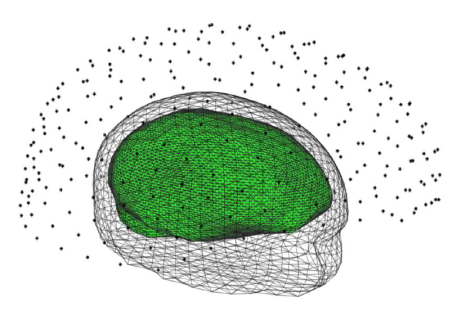
Fig. 1 Head model used in our experiments (only the scalp and the brain are shown). The asterisks indicate the position of the magnetometers above the head

Based on those conditions, the beamformers were evaluated at the position r corresponding to the centroid of each of the triangles comprising the brain mesh. In both cases, the array response matrix A was calculated using the computer implementation provided in²², which corresponds to a solution of based on the boundary element method (BEM) of the quasi-static approximation of Maxwell’s equations. BEM is a numerical method for solving partial differential equations (in this case Maxwell’s equations) with the advantage of reformulating them as discrete integral equations that then are solved on simple geometrical elements of a boundary mesh¹². The data covariance matrix R^ and the noise covariance matrix Q^ were estimated from the data acquired in the 240 ms following the stimulus and the previous 240 ms, respectively. For comparison purposes, we considered the case of l=1 active source in the calculation of MAI and RRMAI_T2.

Figures 2 and 3 show the results of computing the index values for each of the beamformers. Given that the magnitudes of the indexes are very different, we decided to compare them in terms of their distributions. Therefore, we show the histogram of each index, where the red bars indicate the percentiles that were necessary to display so that the positions r with most significant index values (the minimum for the case of the sparsity-based index and the maximum values for the others) had an anatomical correspondence with the expected position neural source. Note that most of the positions indicated with red dots on the surface of the brain’s mesh coincide with a neural activation located at the primary visual cortex, but different portions of the respective distributions of the indexes were accounted for in order to achieve such correspondence. In all cases, we show the mesh modeling the head in an orientation such that the occipital lobe is fully seen from the back of the head.

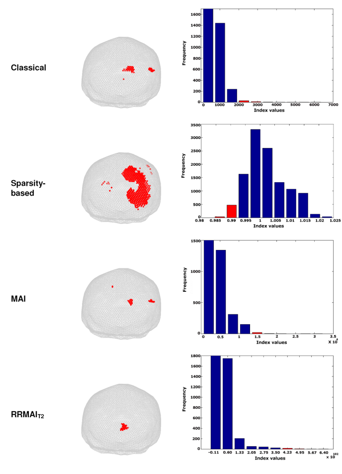
Fig. 2 MEG source localization of a large visual stimulus presented on the left side of the visual field for one subject. The red dots are superimposed in the brain mesh in order to highlight the location of the most significant values of the corresponding index. In the histogram, the red bars indicate the percentile that corresponds with the index values that are displayed

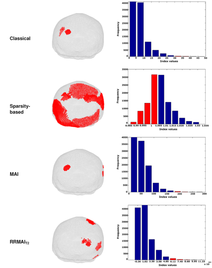
Fig. 3 MEG source localization of a small visual stimulus presented on the right side of the visual field for one subject. The red dots are uperimposed in the brain mesh in order to highlight the location of the most significant values of the corresponding index. In the histogram, the red bars indicate the percentile that corresponds with the index alues that are displayed

In the case of a large visual stimulus presented to the left visual field (Figure 2), both MAI and RRMAI_T2 provide very good results in terms of focalization of the source, but RRMAI_T2 outperforms MAI as its most significant index values correspond with the tail of the distribution. The classical beamformer also achieves good results in those terms, but the position of the estimated source location is biased. Finally, the sparsity-based index is accurate in detecting the region with less-sparse-sources (i.e., those more likely to be related with the stimulus), but fails in terms of focalization. Clearly, an extreme-value distribution would be the most desired outcome in the index calculation process, but the sparsity-based index tends to be better described by a Gaussian distribution.

For a small visual stimulus presented to the right visual field (Figure 3), we obtained similar results as those previously described in terms of the shape of the distributions. However, in this case RRMAI_T2 fails to estimate the source location (an ipsi-lateral patch is detected instead). This can be credited to the fact that we maintained the same value of p in (22) for all our calculations, while it is well-known that such parameter requires to be adjusted in a case-to-case fashion (see¹⁶ for a full account of that issue).

In terms of the computational cost, the calculation of each of the indices here tested was fully implemented in Matlab^®, and the computer used was a HP ProLiant ML110 G7 server with a Xeon E3-1220 processor, 3.1 GHz of speed, and with 6 GB of RAM memory. Under those conditions, computing the sparsity neural index (which is the most mathematically complex of the four) took 42.3095 minutes. Nevertheless, the distance between the two possible solutions (i.e., the distance between the centroids of two triangles sharing a side) was 4.7 millimeters, which is much larger than the allowed error in source localization for clinical applications, such as in neurosurgery, where the sources must be located with a precision of at least 1 mm. Hence, for clinical applications, a much more dense brain mesh (i.e., more triangles in the tessellation) must be used. Still, such increase in the computing complexity is something that can be handled through many different types of hardware (e.g., graphic processing units), and with different algorithms to implement the beamformer (see, e.g., ⁴). In fact, thanks to the increase in computer power, beamforming has been resurrected as a suited technique for analysis of brain activity.

4 Conclusions

The use of spatial filters in the solution of the neuroelectric inverse problem involves very complex mathematical calculations. However, it is possible to manage such calculations with today’s computer power. Furthermore, new spatial filters, such as those based on eigenspace projections, can be used to improve the classical LCMV solution originally proposed in²⁷.

Here, different indices of neural activity (all of them based on beamforming) were compared in terms of their ability to provide a focalized and anatomically correct estimation of a neural evoked response. Therefore, we looked for a beamformer to generate significant index values (i.e., at the tail of the distribution) and with an accurate correspondence with the expected location of the neural activity (primary visual cortex in this case). However, the methods here analyzed showed little consistency, that is, a single method not always provided good results for the same type of data.

Nevertheless, we do not expect to find a spatial filter that performs well for all types of data. For example, in the case of the sparsity-based index, we believe it did not provide good results for the evoked responses here tested as it is better suited for data with low SNR (i.e., with larger sparsity). Another example is the MAI, which is known to perform better for cases where correlated sources are involved, then MAI can be computed within a region-of-interest (ROI) in order to provide a focalized estimation. Therefore, it is necessary to continue with the development of new indexes based on more consistent estimates, as well as characterize the response of different beamformers for different types of data.

Finally, it is worth mentioning that the methods here tested are not mutually exclusive, and information obtained from a combination of methods may improve the overall result. An example of such approach has already been presented in a preliminary version of this paper (see⁶), in which the solutions of the classical neural activity and the sparsity-based indexes were combined in order to increase the focusing in the estimation of auditory evoked responses. Therefore, we believe new techniques in brain source localization may benefit from using hybrid techniques that take advantage of complementary information. Such complementarity could be further extended to the joint analysis of electroencephalographic (EEG) and MEG data. While for this paper only MEG data was available, new acquisition systems allow for the simultaneous measurement of EEG and MEG.

Acknowledgment

This work was supported by the Mexican Council of Science and Technology (Conacyt) through Grant 220145.

References

1. Aine, C. J., Sanfratello, L., Ranken, D., Best, E., MacArthur, J. A., Wallace, T., Gilliam, K., Donahue, C. H., Montaño, R., Bryant, J. E., Scott, A., & Stephen, J. M. (2012). MEG-SIM: a web portal for testing MEG analysis methods using realistic simulated and empirical data. Neuroinformatics, Vol. 10, No. 2, pp. 141-158. [ Links ]

2. Applebaum, S. (1976). Adaptive arrays. IEEE Transactions on Antennas and Propagation, Vol. 24, No. 5, pp. 585-598. [ Links ]

3. Cointepas, Y., Mangin, J.-F., Garnero, L., Poline, J.-B., & Benali, H. (2001). BrainVISA: software platform for visualization and analysis of multi-modality brain data. NeuroImage, Vol. 13, No. 6, pp. 98. [ Links ]

4. El Zooghby, A. H., Christodoulou, C., & Georgiopoulos, M. (1999). A neural-network-based linearly constrained minimum variance beamformer. Microwave and Optical Technology Letters, Vol. 21, No. 6, pp. 451-455. [ Links ]

5. Golub, G. & Van Loan, C. (1996). Matrix Computations. The Johns Hopkins University Press, Baltimore. [ Links ]

6. Gutiérrez, D. (2014). New perspectives on the use of spatial filters in electro/magnetoencephalographic array processing. Encuentro Nacional de Ciencias de la Computacíon. [ Links ]

7. Gutiérrez, D. & Nehorai, A. (2008). Array response kernels for EEG and MEG in multilayer ellipsoidal geometry. IEEE Transactions on Biomedical Engineering, Vol. 55, No. 3, pp. 1103-1111. [ Links ]

8. Gutiérrez, D., Nehorai, A., & Dogandžić, A. (2006). Performance analysis of reduced-rank beamformers for estimating dipole source signals using EEG/MEG. IEEE Transactions of Biomedical Engineering, Vol. 53, No. 5, pp. 840-844. [ Links ]

9. Haimovich, A. M. (1996). The eigencanceler: adaptive radar by eigenanalysis methods. IEEE Transactions on Aerospace Electronics and Systems, Vol. 32, No. 2, pp. 532-542. [ Links ]

10. Hämäläinen, M., Hari, R., Ilmoniemi, R. J., Knuutila, J., & Lounasmaa, O. V. (1993). Magnetoencephalography: theory, instrumentation, and applications to noninvasive studies of the working human brain. Reviews of modern Physics, Vol. 65, No. 2, pp. 413. [ Links ]

11. Juan-Lizandra, M. d. C. (2001). Development and validation of a new method for the adjustment of human brain atlases. Computación y Sistemas, Vol. 5, No. 2, pp. 152-159. [ Links ]

12. Liu, Y., Mukherjee, S., Nishimura, N., Schanz, M., Ye, W., Sutradhar, A., Pan, E., Dumont, N., Frangi, A., & Saez, A. (2011). Recent advances and emerging applications of the boundary element method. Applied Mechanics Reviews, Vol. 64, No. 3, pp. 030802. [ Links ]

13. Malmivuo, J. & Plonsey, R. (1995). Bioelectromagnetism: principles and applications of bioelectric and biomagnetic fields. Oxford University press. [ Links ]

14. Moiseev, A., Gaspar, J. M., Schneider, J. A., & Herdman, A. T. (2011). Application of multi-source minimum variance beamformers for reconstruction of correlated neural activity. NeuroImage, Vol. 58, No. 2, pp. 481-496. [ Links ]

15. Mosher, J. C., Leahy, R., & Lewis, P. S. (1999). EEG and MEG: forward solutions for inverse methods. IEEE Transactions on Biomedical Engineering, Vol. 46, No. 3, pp. 245-259. [ Links ]

16. Piotrowski, T., Gutiérrez, D., Yamada, I., & Zygierewicz, J. (2014). A family of reduced-rank neural activity indices for EEG/MEG source localization. Proceedings of the 2014 International Conference on Brain Informatics and Health, pp. 447-458. [ Links ]

17. Piotrowski, T. & Yamada, I. (2008). MV-PURE estimator: Minimum-variance pseudo-unbiased reduced-rank estimator for linearly constrained ill-condicionted inverse problems. IEEE Trans. Signal Process, Vol. 56, No. 8, pp. 3408-3423. [ Links ]

18. Rogers, A. E., Capallo, R. J., Hinteregger, H. F., Levine, J. I., Nesman, E. F., Webber, J. C., Whitney, A. R., Clark, T. A., Ma, C., Ryan, J., et al. (1983). Very-long-baseline radio interferometry: The Mark III system for geodesy, astrometry, and aperture synthesis. Science, Vol. 219, No. 4580, pp. 51-54. [ Links ]

19. Rohrbaugh, J. W., Parasuraman, R., & Johnson, R. (1990). Event-Related Brain Potentials: Basic Issues and Applications. Oxford Univ. Press, New York. [ Links ]

20. Schmidt, R. O. (1981). A signal subspace approach to multiple emitter location spectral estimation. PhD Thesis, Stanford University. [ Links ]

21. Sekihara, K. & Nagarajan, S. S. (2008). Adaptive Spatial Filters for Electromagnetic Brain Imaging. Springer, Berlin. [ Links ]

22. Stenroos, M., Mäntynen, V., & Nenonen, J. (2007). A MATLAB library for solving quasi-static volume conduction problems using the boundary element method. Computer Methods and Programs in Biomedicine, Vol. 88, No. 3, pp. 256-263. [ Links ]

23. Tadel, F., Baillet, S., Mosher, J. C., Pantazis, D., & Leahy, R. M. (2011). Brainstorm: a user-friendly application for MEG/EEG analysis. J. Computational Intelligence and Neuroscience, Vol. 2011, pp. 8. [ Links ]

24. Van Der Veen, A.-J., Deprettere, E. F., et al. (1993). Subspace-based signal analysis using singular value decomposition. Proceedings of the IEEE, Vol. 81, No. 9, pp. 1277-1308. [ Links ]

25. Van Trees, H. L. (2002). Optimum array processing. Detection, Estimation, and Modulation Theory. Wiley-Interscience. [ Links ]

26. Van Veen, B. D. & Buckley, K. M. (1988). Beamforming: A versatile approach to spatial filtering. IEEE ASSP Magazine, Vol. 5, No. 2, pp. 4-24. [ Links ]

27. Van Veen, B. D., Van Drongelen, W., Yuchtman, M., & Suzuki, A. (1997). Localization of brain electrical activity via linearly constrained minimum variance spatial filtering. IEEE Transactions on Biomedical Engineering, Vol. 44, No. 9, pp. 867-880. [ Links ]

28. Widrow, B., Glover Jr, J. R., McCool, J. M., Kaunitz, J., Williams, C. S., Hearn, R. H., Zeidler, J. R., Dong Jr, E., & Goodlin, R. C. (1975). Adaptive noise cancelling: Principles and applications. Proceedings of the IEEE, Vol. 63, No. 12, pp. 1692-1716. [ Links ]

29. Yamada, I. & Elbadraoui, J. (2006). Minimum-variance pseudo-unbiased low-rank estimator for ill-condicioned inverse problems. Proc. IEEE ICASSP, pp. 325-328. [ Links ]

30. Zaragoza-Martínez, C. C. & Gutiérrez, D. (2013). Electro/magnetoencephalography beamforming with spatial restrictions based on sparsity. Biomedical Signal Processing and Control, Vol. 8, No. 6, pp. 615-623. [ Links ]

Received: August 14, 2015; Accepted: November 25, 2015

Corresponding author is Claudia Carolina Zaragoza-Martinez

Claudia Carolina Zaragoza Martínez received the B.Sc. degree in electronic engineering from the Technological Institute of Madero City, Tamaulipas, in 2009, and the M.Sc. and Ph.D. degrees in biomedical engineering and physics from the Center for Research and Advanced Studies (Cinvestav), Monterrey's Unit, in 2011 and 2015, respectively. Her research interests are in the area of biomedical signal processing, specifically in neurcelectrical signal processing with EEG and MEG data.

David Gutiérrez, better known as Dania Gutiérrez, received the B.Sc. degree (with honors) in electrical engineering from the National Autenemeus University of Mexico (UNAM), Mexico, in 1997, the M.Sc. degree in electrical engineering and computer sciences, as well as the Ph.D. degree in bicengineering from the University of Illincis at Chicago (UIC), in 2000 and 2005, respectively. From March 2005 to May 2006, she held a postdoctoral fellowship at the Department of Computer Systems Engineering and Automation, Institute of Research in Applied Mathematics and Systems (IIMAS), UNAM. In June 2006, she joined the Center for Research and Advanced Studies (Cinvestav) at Monterrey, Mexico. There, she is an asscciate professor in the area of medical sciences, as well as the current academic secretary. Dr. Gutierrez's research interests are in statistical signal processing and its applications to biomedicine. She is also interested in computer sciences, neurosciences, and robotics. Dr. Gutierrez is a former Fulbright Scholar, and a former student fellow of the Mexican Council for Science and Technclogy (Conacyt). She has been a member of Conacyt's researchers system (SNI) since 2007, from which she currently holds the Level-I fellcwship. She is also a Senior Member of the Institute of Electrical and Electronics Engineers (IEEE).

This is an open-access article distributed under the terms of the Creative Commons Attribution License