


 nueva página del texto (beta)
 Inglés (pdf)
 Artículo en XML
 Referencias del artículo
 Enviar artículo por email
 Citado por SciELO
  Similares en
SciELO
Similares en
SciELO 
 Permalink
1. Introduction
In the geophysics forward modeling context around the oil wells, the electric resistivity is a parameter that plays an important role. The Marine Controlled-Source Electromagnetic Method (CSEM) has emerged as a useful exploration technique for mapping offshore hydrocarbon reservoirs and characterizing gas hydrates bearing shallow sediments 4. In a standard configuration, the Marine CSEM uses a deep-towed horizontal electric dipole (HED) to transmit electromagnetic signals into the seawater and sediments below the mudline23.
An edge-based parallel code for numerical simulation of marine CSEM surveys in 3D isotropic structures is presented. In order to represent complex bodies with high fidelity we used unstructured tetrahedral meshes. The heart of our computational solution is based on the Edge Finite Element Method (EFEM) because it has the ability to eliminate spurious solutions and is claimed to yield accurate results. The framework structure is able to exploit the embarrassingly-parallel tasks, or tasks where there is no dependency (or communication) between those parallel tasks, and the advantages of the geometric flexibility as well as to work with three different orientations for the dipole (HED).
Marine CSEM response for a single HED at a single frequency requires a forward modeling whose computing can easily overwhelm single core and modest multi-core computing resources17. In fact, the actual execution of real-life scale simulations of electromagnetic geophysical problems requires using HPC because typical executions involve over 100,000 realizations, each dealing with several millions of degrees of freedom. To alleviate these issues, our parallel work-flow is focused on such edge tasks as the edges-elements array connectivity, the edge data computation (length, unit vector, local/global edge direction), physical properties at each edge (electric resistivity, primary electric field), and the electric field interpolation.
Regarding the computational burden, only six unknowns are required for each element (Nédélec tetrahedral elements of lower order). It is worth nothing that the linear vectorial Lagrange elements or any other consistently linear 3D-vector functions over a tetrahedral carry twelve unknowns, three at each of its four vertices. However, the state of the art is marked by a relative scarcity of robust edge-based codes to simulate these problems. This may be attributed to the fact that not all numerical approaches are well-suited for the latest computing architectures. For that reason, the software stack presented here was designed taking into account an architecture-aware approach.
We structure the paper as follows: in Section 2 we describe the background theory of marine CSEM. In Section 3 we present the formulation of electromagnetic (EM) field equations in isotropic domains. Parallel framework is described in Section 4. The performance and efficiency of the code are investigated using a 3D canonical model in Section 5. All experiments were performed on the Marenostrum supercomputer with two-8 cores Intel Xeon processors E52670 at 2.6 GHz per node. The last section is dedicated to conclusions.
2. Marine Controlled-source Electromagnetic Method
The Marine Controlled-source Electromagnetic Methods (CSEM) are a type of geophysical strategies to study the subsurface electrical conductivity distribution with an ample range of applications. CSEM techniques can be divided into two groups depending on the domain in which the collected data is interpreted: time domains (TDEM) or frequency domains (FDEM). In the case of oil prospecting, marine CSEM surveys are done predominantly using FDEM2,14.
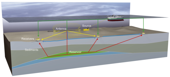
In the marine CSEM, also referred to as seabed logging12, a deep-towed electric dipole transmitter is used to produce a low frequency EM signal (primary field) which interacts with the electrically conductive Earth and induces eddy currents that become sources of a new EM signal (secondary field). The two fields, the primary one and the secondary one, add up to a resultant field, which is measured by remote receivers placed on the seabed. Since the secondary field at low frequencies, for which displacement currents are negligible, depends primarily on the electric conductivity distribution of the ground, it is possible to detect thin resistive layers beneath the seabed by studying the received signal15. Operating frequencies of transmitters in CSEM may range between 0.1 and 10 Hz, and the choice depends on the model dimensions. In most studies, typical frequencies vary from 0.25 to 1 Hz, which means that for source-receiver offsets of 10-12 km, the penetration depth of the method can extend to several kilometers below the seabed1,4,6,15.
The disadvantage of the marine CSEM is its relatively low resolution compared to seismic imaging. Therefore, the marine CSEM is almost always used in conjunction with seismic surveying as the latter helps to constrain the resistivity model. Figure 1 depicts the marine CSEM which is nowadays a well-known geophysical prospecting tool in the offshore environment and a commonplace in industry; examples of that can be found in 9,10,18,14,22.
The Marine CSEM is a viable and cost-effective oil exploration technique. When integrated with other geophysics data, mainly, seismic information, CSEM surveys are promising for adding value in shallow/deep waters. The outcomes and analysis of modeling with CSEM produce a more robust understanding of the prospection.
3. Edge Finite Element Approximation
The 3D EM modeling requires solving diffusive Maxwell equations in a discretized form. The most popular numerical methods for EM forward modeling are Finite Difference (FD), Finite Element Method (FEM), and Integral Equation (IE). Among them, the FEM is more suitable for modeling EM response in complex geometries. However, for accurate computations, the divergence free condition for the EM fields in the source free regions needs to be addressed by an additional penalty term, commonly called Gauge condition, to alleviate possible spurious solutions13,15.
As a result, in FEM the use of Edge-based FEM (EFEM), also called Nédélec elements, has become very popular for solving EM fields problems. In fact, EFEM is often said to be a cure for many difficulties that are encountered (particularly eliminating spurious solutions) and is claimed to yield accurate results13,16,21. The basis functions of Nédélec elements are vectorial functions defined along the element edges. The tangential continuity of either electric or magnetic field is imposed automatically on the element interfaces while the normal components are still can be discontinuous . As a result, EFEM has the capability to model the frequency/time domain EM fields in inhomogeneous complex bodies at any resistivities contrasts and at any survey types. Therefore, our code is based on the Nédélec elements formulation by 7,8.
In geophysical applications, the low frequency EM field satisfies the following Maxwell’s equations:
where we adopt the harmonic time dependence
In EM field formulations with FEM and EFEM and in order to capture the rapid change of the primary current, the anomalous formulations are desirable 5. In the anomalous field formulation the total field is decomposed into primary field (background) and secondary field 24:
Based on this formulation, one can derive the following equation for the secondary electric field:
In 5, the source term is the primary electric field, which is much smoother than the source current. In this sense, our formulation is able to work with three different orientations for the HED, which are given by 8.
Therefore, the primary field is calculated analytically using a horizontal layered-earth model and the secondary field is discretized by linear Nédélec elements. For this purpose, we first replace the following continuous condition:
fixing the normal component
stating that 6 is satisfied on average on each face element of Ω. We end up in all cases with one or several relations linking the integral of
where r
i are the edges of the boundary
where the coefficients
Homogeneous Dirichlet boundary conditions are applied to the outer boundaries of the model. The EFEM discretization results in a linear equation system, which is solved using the iterative Quasi Minimal Residual Method (QMR) and the Biconjugate gradient Method (BCG) 3.
4. Framework
Despite the popularity of the EFEM, there are few implementations of it. Furthermore, the 3D modeling of geophysical EM problems can easily overwhelm single core and modest multi-core computing resources 17. In fact, the actual execution of real-life scale simulations of electromagnetic geophysical problems requires using HPC because typical executions involve over 100,000 realizations, each dealing with several millions of degrees of freedom. To alleviate these issues, our parallel framework is able to exploit the embarrassingly-parallel tasks, or tasks where there is no dependency (or communication) between those parallel tasks.
Figure 2 shows the software stack of our solution. Specific details and features of each module are as follows.
Mesh. This module reads geometric and topological properties of an FEM mesh: how the elements are connected and where their nodes are located. Our implementation is able to read as input nodal-based meshes in three different formats: Netgen, Gambit, and Neutral format 7.
Mesh refinement. To increase the solution accuracy, our framework uses a uniform refinement. In tetrahedral meshes, this approach results in 8 times more tetrahedral elements.
Counterclockwise numbering. In order to get a consistent notation in the whole domain, this module sets the node numbering within each element in a counterclockwise direction.
Edges computation. In EFEM formulations, the unknowns are associated to edges instead of the nodes. Because most of the FEM codes were developed for node-based formulations, it is necessary to develop a code to convert node numbering into edge numbering. Therefore, this module computes a matrix to represent every element by its edges and other matrix to describe every edge by its two nodes with dimensions (6 x TT) and (2 x TE), respectively, where TT is the number of elements and TE is the total number of edges. These matrices define the global/local edge direction in the mesh 7,13.
Primary field computation. This module computes the primary field on each edge according to the formulation in 8. Furthermore, this module computes others edge values such as edge length and unit edge vector, which are critical for the interpolation stage, through the vector basis functions defined in 7,8.
-
Sigma edges computacion. This module computes the sigma value for each edge. In the formulation of our geophysical application, this operation can be summarized by the following expression:
where
Assembly. This module assembles the system matrix whose general form is Ax = b. In electromagnetic simulations, and particularly in geophysical prospecting through EM such as CSEM, the matrix A is large, sparse, complex, and symmetric; the vector x contains the unknowns coefficients, and the vector b stores the contributions of the primary field. To exploit special properties of EFEM matrices, the parallel assembly process uses a Compressed Row Storage (CRS).
-
Boundary conditions (BC). Before the system of equations is ready to be solved, the imposition of BC is needed. Actually, our code works with Dirichlet BC and their imposition is accomplished by setting 13
for j ≠ ind(i) , where ind(i) is a vector that stores the global edge indexes residing on the boundaries, and v(i) is a vector that contains the prescribed values of x. Different techniques are described in 9.
Solver. In FEM or EFEM applications, the solvers are frequently iterative, but sometimes one may also want to use direct solvers. This module is able to work with two iterative solvers: BCG and QMR. Since the framework is based on an abstract data structure, it is possible to use other solvers with little effort.
Interpolation. This module computes the electric response for an array of receivers. The interpolation process uses the vectorial functions defined in 7,8 because these automatically enforce the divergence free conditions for EM fields. Moreover, the continuity of the tangential EM is satisfied automatically.
Output. Once a solution of EFEM problem on a given mesh has been obtained, it should be post-processed by using a visualization program. Our framework does not do the visualization by itself, but it generates output files (vtk format) with the final results. It also gives timing values in order to evaluate the performance.
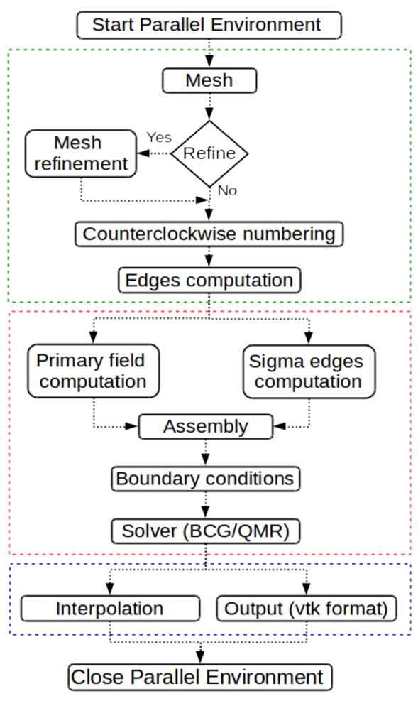
Fig. 2 Software stack. Green dashed: pre-processing stage, red dashed: forward modeling, blue dashed: post-processing stage
In order to meet the high computational cost of EFEM for EM fields in geophysical applications, actually our code is based on a shared memory parallel model defined by the OpenMP standard 20. OpenMP has been widely adopted in the scientific computing community, and most vendors support its Application Programming Interface (API) in their compiler suites. OpenMP offers not only parallel programs portability but, since it is based on directives, it also represents a simple way to maintain a single code for the serial and parallel version of an application.
To exploit the advantages of geometric flexibility, our parallel approach is focused on embarrassingly parallel tasks, or tasks where there is no dependency (or communication) between those parallel tasks. Namely, the minimum level of computing work is related to the edges in the mesh. Examples of embarrassingly parallel modules are computation of edges, primary field computation, and sigma edges computation. Another parallel task is interpolation, the only difference lies in the parallelism level because it works over the number of receivers (points) instead of the number of edges.
A detailed description of the main algorithms of our code can be found in 8.
5. Results
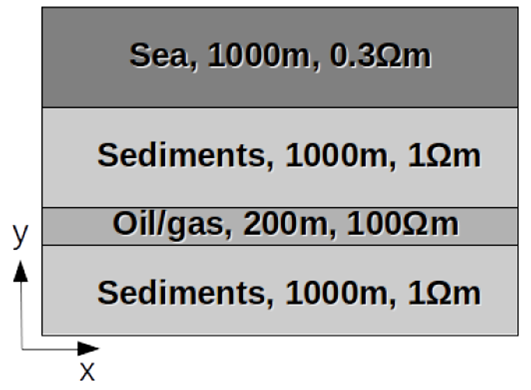
To verify the accuracy and performance of our modeling, we used the model defined in Figure 3. Our code is able to work with three different dipole’s orientations (x-oriented, y-oriented and z-oriented) according to the formulation in 7),(8. This source transmits a carefully designed low-frequency EM signal into the subsurface. The main physical parameters for our test are described in Table 1.

The experiments were performed on the Marenostrum supercomputer with two-8 cores Intel Xeon processors E52670 at 2.6 GHz per node. To increase the solution accuracy, our implementation used a non-uniform refinement.
Table 2 summarizes the results of our tests. For each experiment, the problem size stays fixed but the number of processing units is increased (the strong scaling approach). The parallel efficiency is given by

From the results in Table 2 it is easy to see that in our experiments the minimum execution time is not limited by the communication overhead, as a result, we achieved a quasi linear speed-up. The latter issue is critical because if the computation time in each processor is smaller than the communication time, the speed-up can saturate. Table 2 also shows the total number of tetrahedral elements (TT) and the total number of edges (TE), which is a measure of required storage space during run-time. TT and TE were determined by successively refined meshes.
In order to validate our numerical formulation, the components of Ee obtained from equation 3 versus components of
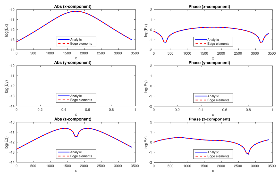
Fig. 4 Total electric field components. Comparison between solution Eh (edge elements) from Test 5 and the exact solution Ee (analytic)
In Table 3 we show the errors for the components of
Table 3 Errors in L1-norm, L2-norm, and L∞-norm for solution Eh with respect to the exact solution Ee

Errors in Table 3 demonstrate that edge elements of lower-order reach the desired accuracy when the number of edges is increased (TE or dofs in the mesh).
6. Conclusions
The electromagnetic methods are an established tool in geophysics, finding application in many areas such as hydrocarbon and mineral exploration, reservoir monitoring, CO2 storage characterization, geothermal reservoir imaging, and many others. In particular, the marine CSEM has become an important technique for reducing ambiguities in data interpretation in hydrocarbon exploration.
Considering the societal value of exploration geophysics, we presented an edge-based parallel code for the forward modeling of the marine CSEM in 3D isotropic structures. The framework is based on unstructured tetrahedral meshes because these have the ability to represent complex bodies with high fidelity. The heart of our computational solution is based on EFEM because it can eliminate spurious solutions and is claimed to yield accurate results.
Recent trends in parallel computing techniques were investigated for their use in mitigating the computational overburden associated with the electromagnetic modeling. Therefore, our parallel work-flow is focused on such edge tasks as edges-elements array connectivity, edge data computation (length, unit vector, local/global edge direction), physical properties at each edge (electric resistivity, primary electric field), matrix assembly, and the electric field interpolation. As a result, we obtained a parallel framework whose main modules are flexible and simple.
Concerning the computational burden, only six unknowns are required for each element (Nédélec tetrahedral elements of lower order). It is worth noting that the linear vectorial Lagrange elements or any other consistently linear 3D-vector functions over a tetrahedral carry twelve unknowns, three at each of its four vertices. In addition, the software stack presented here was designed taking into account an architecture-aware approach.
The efficiency and accuracy of the code were evaluated through scalability tests (strong scaling) and error-norms for different mesh sizes. The results show not only a good parallel efficiency of our code but also an acceptable accuracy in the numerical approximation.
All the experiments were performed on the Marenostrum supercomputer at the Barcelona Supercomputing Center (www.bsc.es).
Future work will be aimed at the implementation of the anisotropy cases and at application of MPI communications which are needed to use distributed memory platforms.

