


 text new page (beta)
 English (pdf)
 Article in xml format
 Article references
 Send this article by e-mail
 Cited by SciELO
  Similars in
SciELO
Similars in
SciELO 
 Permalink
1 Introduction
Minimum-phase (MP) filters find applications in communications, speech processing, and predictive coding, among others 1, 4. The special feature of an MP filter is that it does not contain zeros outside the unit circle. As a consequence, an MP filter has several important and interesting properties revised in Section 2.
There exist two main approaches for MP filter design:
The design of an MP FIR filter starting from a low-pass FIR prototype has many advantages 5. The methods consist of the FIR prototype design and finding all zeros of the designed filter. In the next step, all zeros which are outside the unit circle are reflected to their reciprocal positions inside the unit circle. This process is called mipizing 5.
We consider here the MP FIR filter design based on LP FIR prototype design and mipizing. In our previous work 8 we proposed the IFIR (interpolated finite impulse response) filter for the design of MP filters. The sharpening technique for the design of MP filters is considered in 9, 10.
Specifically, we propose a novel procedure for the design of high order MP filters based on low complexity FIR filters using the sharpening and the IFIR techniques. We also introduce the rules for sharpening IFIR MP filters.
The paper is organized in the following way. The next section gives a brief review of mipizing and properties of MP filters. A review of IFIR filters and the sharpening technique is given in Section 3. The rules for the MP IFIR sharpening are described in Section 4. Section 5 presents the steps for the MP filter design based on the rules established in Section 4. The algorithm is illustrated with one example. Finally, the comparison with existing methods is provided in Section 6 to demonstrate the benefit of the proposed design. Finally, the conclusions are given in Section 7.
2 Mipizing and Properties of MP Filters
Mipizing consists in reflecting the zeros of LP FIR filter to their reciprocal positions inside the unit circle. This process does not change the magnitude response of the filter 4, as illustrated in the following example.
Example 1. We consider the MP filter design based on mipizing of LP FIR prototype filter, which satisfies the following specification: the normalized pass-band frequency ωρ = 0.1, the normalized stop-band frequency ωs = 0.25, the pass-band ripple is of 0.1 dB, and the minimum stop-band attenuation is of 60 dB.
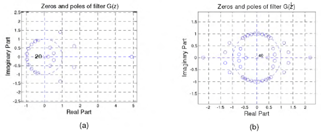
The filter is designed in MATLAB using Remez algorithm. The obtained LP filter has an order of Ν = 36. The plot of its zeros is shown in Fig. 1 (a). There are three zeros outside the unit circle.
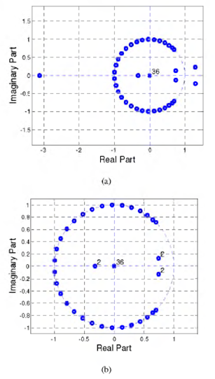
Mipizing consists in reflecting those zeros to their reciprocal positions, as shown in Fig. 1 (b). Next, the zeros of the MP filter are converted to the polynomial using the MATLAB file poly.m. The polynomial coefficients correspond to the impulse response coefficients.
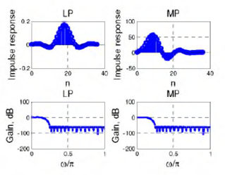
Fig. 2 shows the corresponding impulse and gain responses. Note that the gain responses of LP filter and the mipized filter are equal.
The MP filters have a number of interesting and important properties 4 illustrated in the following subsection using the filters from Example 1.
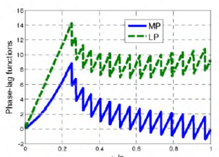
2.1 The Minimum Phase-Lag Property
Mipizing decreases the phase-lag function (the negative of the phase), as shown in Fig. 3.
2.2 The Minimum Energy Delay Property
The partial energy of MP systems is most concentrated around n=0,
 1
1
where hm(n) and h(n) are impulse responses of the MP and LP filters, respectively. For this reason MP filters are also called minimum energy delay systems.
The group delay (grd) of a system Η(ejω) is defined as a negative derivation of the corresponding phase:
 2
2
The group delay of an MP system is always less than that of non-minimum phase systems having the equal magnitude responses, as shown in Fig. 4.

3 Review of IFIR and Sharpening
The IFIR filter technique designs a more complex LP filter using two less complex filters 15. The structure of an IFIR filter is shown in Fig. 5.
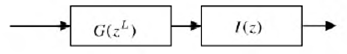
The model filter G(z) is designed using the following specification 15:
where ωρ and wsare the pass-band and stop-band frequencies, RP is a maximum pass-band ripple, and As is a minimum attenuation of the prototype filter.
From (3), it follows that the transition band is L times higher than that of the prototype filter, resulting in approximately L times less order of the model filter. Next, the model filter is expanded by a factor L, becoming G(zL), so that the specification of the model filter coincides with that of the prototype filter. In this process, each delay z 1 of the designed filter G(z) is replaced by zL, or alternatively, L-1 zeros are inserted between the consecutive samples of the impulse response of the filter G(z). However, the changing from G(z) to G(z L ) has a consequence that L-1 images of the original spectrum are introduced between 0 and 2π. That is the reason why one needs another filter called interpolation filter /(z), which has to eliminate images introduced by G(z L ). The specification of the filter /(z) is given as 15:
More details can be found in 15.
The sharpening technique is introduced in 16 for simultaneous improvements of both the pass-band and stop-band of a linear-phase FIR filter. The sharpening technique uses the amplitude change function (ACF) which is a polynomial relationship of the form Ηsh = f(H) between the amplitudes of the sharpened and the prototype filters, Hsh and H, respectively.
The improvement in the gain response near the pass-band edge H=1, or near the stop-band edge H=0, depends on the order of tangencies m and n of the ACF at H=1, or at H=0, respectively.
We will consider here the most popular sharpening polynomial (m=1, n=1):
However, the sharpening technique can only be applied to LP filters. In 10 it is shown how the sharpening can be applied to MP filters. In this paper we show how we can also apply sharpening to MP IFIR filters.
4 Rules for Sharpening and Mipizing IFIR filters
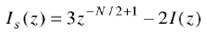
Sharpening of an IFIR filter is practically equivalent to the cascade of sharpened expanded model and interpolation filters:
where Sh{.} means sharpening.
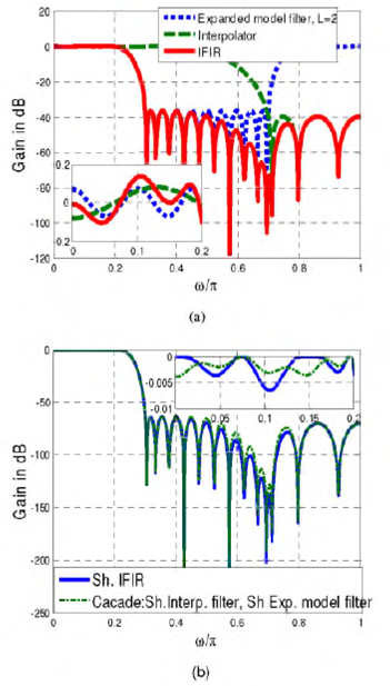
Example 2. The IFIR filter is designed satisfying the following specification: ωρ=0.2, ω5=0.3, Z=2, Rp=0.2dB, As=40dB.
Fig. 6 (a) shows the gain responses for the expanded model, interpolation, and IFIR filters. Similarly, Fig. 6 (b) compares the sharpened filters from left and right sides of (6).
The sharpening of interpolation and expanded model filters can be presented in the following forms 10:
 7
7
 8
8
where
 9
9
 10
10
From (9) and (10), it follows that the order Ν of both model and interpolator filters must be even. The corresponding impulse responses are
 11a
11a
 11b
11b
 12a
12a
 12b
12b
In what follows we explain how to obtain the corresponding MP filters from (9) and (10).
4.1 Expanded Filter Roots
In the expanded filter, each zero of the original filter zi = ri ejψ is mapped into L zeros 8.
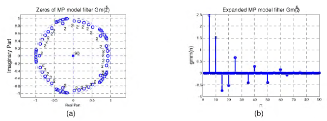
As an example, Fig. 7 presents zeros of the model filter G(z) and the corresponding expanded filter G(zL), for Z=2.
The mipizing of the expanded filter can be performed in two steps:
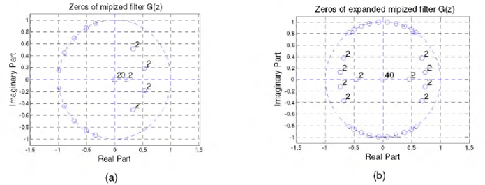
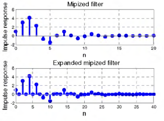
Fig. 8 (a) shows zeros of the mipized filter G(z), while Fig. 8 (b) shows the zeros of the mipized expanded filter. Fig. 9 presents the corresponding impulse responses obtained using MATLAB file poly.m.
4.2 Rouche's Theorem
We apply the Rouche's theorem 17 to find the number of zeros inside the unit circle for polynomials Gs(z) and ls(z). The theorem states the following 17: "Let f(z) and g(z) be analytic functions inside and on a positively oriented simple closed contour C, and if \f(z)\ > \g(z)\ at each point z on C, the functions f(z) and f(z)+ g(z) have the same number of zeros, counting multiplicities, inside C."
To this end we rewrite Gs(z) as
 14
14
We denote
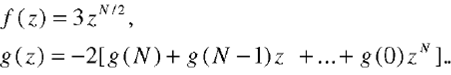 15
15
The corresponding absolute values are
 16
16
Considering that the contour C is a unit circle, we have |z|=1, resulting in
 17
17Observe that the condition in Rouche's theorem is satisfied because
 18
18
on the unit circle.
Since f(z) has N/2 zeros, counting multiplicities, interior to the unit circle |z|=1, the polynomial f(z)+g(z), or Gs(z) has also N/2 zeros inside the unit circle. Knowing that the filter Gs(z) is a linear-phase filter, the rest of its N/2 zeros are outside the unit circle in the reciprocal positions of zeros that are inside the unit circle.
Similarly, we can also show that half of zeros of a linear-phase filter ls(z) are inside the unit circle, and the other half of zeros are in the reciprocal positions, i.e., outside the unit circle.
These statements result in a simple rule for the mipizing the filters Gs(z) and ls(z):
-Eliminate zeros outside the unit circle, and double the zeros which are inside the unit circle.
5 Description of the Method
The sharpened MP filter Hm(z) is obtained using the results from section 4 as
 19
19
Where
Gm (zL) is the mipized expanded model filter.
lm(z) is the mipized interpolation filter.
Gsm(z) is the mipized filter Gs(z).
Ism(z) is the mipized filter ls(z).
The procedure for the design is described in the following steps:
Step 1. Design the model filter G(z) and the interpolator l(z) according to the given specification.
Step 2. Mipize the filters G(z) and l(z) in order to obtain the MP filters Gm(z) and lm(z).
Step 3. Obtain the expanded filter Gm(zL) from the MP filter Gm(z).
Step 4. Using (11) and (12), find the LP filters Gs(z) and ls(z).
Step 5. Delete all zeros of Gs(z) and U(z) which are outside the unit circle, and double those which are inside.
Step 6. Find Gsm(z) and lsm(z).
Step 7. Using (19), find the sharpened IFIR MP filter.
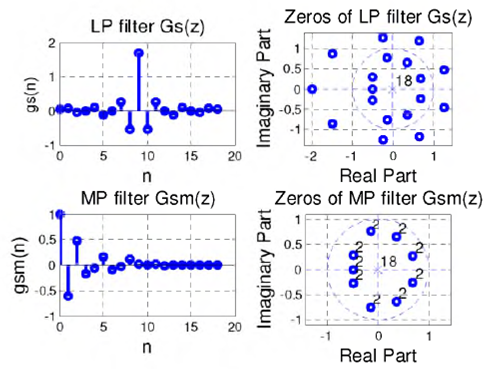
Example 3. We illustrate the method by sharpening the IFIR filter which satisfies the following specification: ωρ=0.12, ωs=0.15, L=5, Rp=1dB, As=38dB.
Step 1. We design the model and interpolation filters and find their zeros, as shown in Fig. 10. The orders of the model and interpolation filters are 18 and 24, respectively, and the conditions in (9) and (10) are satisfied. Observe that the orders of filters are even.

Step 2. We mipize the model and interpolation filters, as shown in Fig. 11.

Step 3. Expand the filter Gm(z) using (13). Fig. 12 shows the zeros and impulse response of the MP expanded model filter.
Step 4. Find LP filters Gs(z) and ls(z).
Step 5. Find the zeros of the LP filters Gs(z) and ls(z) and the zeros of the corresponding MP filters Gsm(z) and l sm(z), as shown in Figs. 13 and 14.

Step 6. Find the corresponding polynomials Gsm(z) and l sm(z).
Step 7. Using (19), find the sharpened IFIR MP filter.
Fig. 15 compares the gain responses of MP IFIR and MP sharpened IFIR filters. Note that the resulting MP filter has approximately 50% more stop-band attenuation and two times less pass-band ripple than the MP IFIR filter.
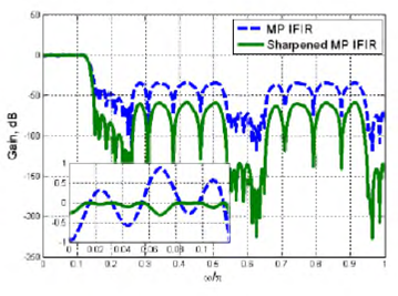
The corresponding MP filter obtained by mipizing an LP equiripple FIR filter has an order of 158. However, in the proposed design, the MP filter is obtained using filters of orders 18 and 24.
6 Comparison with the Method in ( 4 )
Finally, we compare our proposed design with the method described in 4, which uses the cepstrum technique. Fig. 16 shows the resulting gain responses. Observe that our proposed approach has better gain response than the approach given in 4. It is worth to point out that our approach is based on the design of low order digital filters, while method in 4 is based on the design of a high order FIR filter and the complex cepstrum technique.

7 Conclusions
A simple procedure for sharpening MP FIR filters is presented. It is demonstrated that the sharpening and IFIR design techniques, developed for LP narrow-band filters, can also be used for the MP narrow-band filter design. The only restriction is that the orders of the model and interpolation filters must be even.
Additionally, our method, like the IFIR technique, is useful not only for lowpass filters but also for highpass and certain bandpass filters, by a simple change of the specification of the corresponding interpolation filter. The filters are designed using MATLAB Remez algorithm and the files roots.m and poly.m. This work is devoted to the design of narrow-band MP filters. As a future work, we consider the design of minimum phase filters using frequency masking approach 2, which can be used to design wideband minimum-phase filters.

