


 text new page (beta)
 English (pdf)
 Article in xml format
 Article references
 Send this article by e-mail
 Cited by SciELO
  Similars in
SciELO
Similars in
SciELO 
 Permalink
1 Introduction
Micro finance institutions (MFIs) attempt to reduce poverty and income inequality by making credit and other financial instruments accessible to underprivileged, poor populations, thus the number of people that start small businesses within this socio-economical group can increase. MFIs are popular in underdeveloped countries, but the challenge of these enterprises is to remain profitable despite the high risk associated with their investments. Penetrating the market by establishing a certain number of branches of the MFI to serve a given customer base is a critical business decision. This includes the selection of the location and type of the territory centers from potential branches and allocation of the customer base to these territory centers with respect to particular planning criteria. We utilize the two-phase location-allocation optimization approach that was proposed in 1 in order to construct a multi-criteria territory design for a single MFI. This model considers both the mean and variance of a planning criterion. In order to solve the resulting large scale mixed integer program, we utilize a number of heuristics within a branch and bound framework. This manuscript focuses on the comprehensive statistical analysis that provides insights about the interplay of the heuristics. We discuss the effect of the proposed heuristics on the solution quality and computational time in order to provide insights about their use in the solution of mixed integer programs with large scale instances.
1.1 The Literature on Micro Finance Institutions
The MFI literature is vast in decision-making models that focus on measuring efficiency. For example, Data Envelopment Analysis (DEA) has been used extensively with different criteria to measure the efficiency of MFI. The review in 2 provides a discussion about these approaches, while 3 proposes an approach based on Goal Programming that simultaneously considers the effects of multiple criteria involved in the performance of MFI. To the best of our knowledge, there are no models dealing with territory design for MFIs. In fact, territory design problems are relatively scarce in the banking literature. For instance, facility location problems for banking are reviewed in 4. A budget-constrained location model that simultaneously opens and closes facilities is developed in 5 to satisfy customer demand. These authors use greedy-interchange, tabu search, and Lagrangean relaxation heuristics for solving the model. A local search heuristic to solve the mixed integer program of locating bank branches is proposed in 6.
1.2 Territory Design Optimization
Optimization models for territory design have been proposed in applications related to geography, political science, sales, and public resource management. According to 7, territory design criteria can be based on activity-related, organizational, or geographical considerations. The territory design model of 8 minimizes the traveling distance subject to geographical constraints in a sparse environment. Activity-related criteria motivated by economic indicators (i.e. number of customers, demand, workload, sales, and profit) are studied in 9,13. Multi-criteria optimization models have also been considered for territory design. The authors of 14 propose a location-allocation model that balances the number of customers, product demand, and workload while considering connectivity constraints.
The use of activity measures for territory design is restricted to the use of their mean values. The variability of activity measures has not been considered in the existing literature. The research in 1 addresses this gap by utilizing the formulation in 15, which is similar to the quadratic mixed integer mean-variance portfolio selection model of 16. This allows the decision maker to consider the variance of the activity measure, profit allocation, which is a novelty in territory design models. The integer and binary decision variables within territory design problems make mixed integer programs (MIP) a natural choice for modeling. When the size of the problem increases, finding optimal integer solutions is difficult because of the NP-hard characteristics and particular constraints. For instance, enumeration of the exponential number of connectivity constraints becomes practically impossible, see 17. It is also prohibitive in terms of time to solve the resulting MIP for large size instances. Therefore, heuristics have been utilized to deal with such models. Heuristics may not provide perfectly optimal solutions, but they result in sub-optimal decisions within reasonable computational times, thus they are effective for solving real-world problems with large size instances. In 18, the proposed solution for territory design MIP problems ranges from location-allocation and set partitioning methods to divisional algorithms, local search methods, and meta-heuristics.
The proposed heuristics for territory design problems include fixing the locations of the centers, limiting the search to immediate neighborhood, fixing some binary values of variables, perturbation analysis. The authors of 14 propose a reactive greedy randomized adaptive search procedure, and 10 presents a procedure using quadratic models to solve problems with double balancing and connectivity constraints. A similar framework is used in 12, but their focus is on the allocation phase for larger number of instances. In addition to the heuristics that are proposed by 19, heuristics for dynamic re-calculation for profit variance among territory centers and dynamic relocation of branches are introduced and tested. The rest of the manuscript is structured as follows. Section 2 describes the territory design problem, the model formulation, and the data. Section 3 introduces the solution framework and the utilized heuristics. In Section 4, the experimental design is described, whereas the empirical evaluation of the proposed heuristics is given in Section 5. Section 6 presents conclusions and future work.
2 Problem Description, Modeling Framework, and Data Description
2.1 Problem Description
The MFI of concern, as illustrated in Figure 1, offers three major loan products: personal loans, family loans, and group loans. The MFI branches are fully contained within other established businesses. That is, each branch is located inside or adjacent to businesses that attract a large volume of customers and have convenient locations. In our setting, five types of branches are considered, including branches fully contained in grocery stores, convenience/meat markets, drug stores, gas stations, and fast-food restaurants. This configuration enables the firm to reduce the branches' building and operating costs.
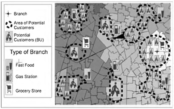
The group of customers that are served by a branch is referred to as a territory. Furthermore, the optimal territory center is the branch that minimizes the total distance of the customers assigned to that particular branch. The problem requires constructing an overall optimal territory design for ρ branches that also satisfies the constraints for the activity measures of interest.
The MFI has a large base of customers; hence, individual customers are aggregated in basic units (BU) to reduce the problem size and model complexity. In the MFI under analysis, each BU is defined so it has at most 15 customers. Each BU has a capacity for the types of branches that it can get service from, whereas each branch is capable of servicing one or more basic units.
2.2 Modeling Framework
We have a territory design problem that can be modeled in one stage as a large facility location problem with the requirement of allocation with respect to different activity measures. To facilitate the solution framework, we propose a two phase location-allocation model. The location model provides the decision on the location and type of the territory centers, whereas the second phase allocates the customers to these territory centers with respect to such activity criteria as the total workload, total dollar amount of loans, and total profit contribution while allowing the initial locations to be updated. Below, we introduce the sets, parameters, decision variables, and activity measures used in the proposed model.
Sets for Model Phases I and II:
A = set of activity measures for BU; indexed by m
Β = set of type of branches {grocery, meat store, drug, gas station, fast-food}; indexed by b
V = set of all available BU's
Ρ = set of disjoint territories; a subset of V
Ε = set of previous customer assignments to branches (i.e. alignment information)
F = sub-set of pairs of BU's that cannot be assigned to the same territory
D = set of connected BU pairs with Euclidean distances D j between BU i and BU j
N j = set of all BU's that are adjacent to j h BU
C = set of unconnected BU's assigned to each territory center
N c = union set of all BU's that are adjacent to any member of C
Parameters for Phases I and II:
v = number of BU's seeking for loan,
ρ = # of branches selected as territory centers,
v = number of BU's seeking for loan,
ρ = # of branches selected as territory centers,
m = # of activity measures among branches,
b= number of branch types,
l = number of loan types,
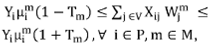
Wjm = value of activity measure m for BUj,
Wjm = value of activity measure m for BUj,
Tm = territorial tolerance for activity measure m,
PVj = variance of the profit for BUj;
Yi = target profit variance for branch i,
Dij = Euclidian distance between BUi and BUj,
Mij = binary parameter for existing assignments if
BUj is assigned to branch i,
δi = maximum travelling distance for customers assigned to branch i,
Gib = binary parameter: {1} if branch i is of type b,
Lb = minimal # of branches selected of type b,
Ub= maximal # of branches selected of type b.
Activity Measures:
m=1. Total workload (in hours per day) required for end-customers.
m=2. Total dollar amount of loans for end-customers.
m=3. Total profit contribution due to accrued interests for end-customers.
Decision Variables for Phases I and II:
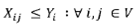
Xij ∀ i,j ∈V, X ij , where {(i,j)} ⊂ D; binary variable indicating if BU j is assigned to branch i,
Y t : ∀ ∈ V binary variable indicating if i th branch is defined as territory center,
Si ∀ ∈ V excess profit variance for branch i when compared with target γ i .
2.3 Phase 1. MIP Model for Initial Territory Centers Location
Phase 1 of the model determines the initial location of the territory centers. Our location MIP model is presented as follows
 PI.1
PI.1
Subjet to
 PI.2
PI.2
 PI.3
PI.3
 PI.4
PI.4
 PI.5
PI.5
Objective Function: we implement a p-median location model with the objective function (PI. 1) minimizing the sum of the Euclidean distances between each BUj and its center BUi. Hence, minimizing dispersion is equivalent to maximizing compactness. The set V(set of all available BU's) can be partitioned into the set of ρ disjoint territories, P. The objective function finds the initial location and type of ρ branches to be selected as territory centers.
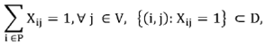
Unique assignment constraint: constraint (PI.2) assigns each BUj to only one branch.
Capacity constraints: constraint (PI.3) assigns BUj to branch i if and only if branch i is selected as a territory center. Constraint (PI.4) provides a lower bound for branch i assignments in terms of activity measures.
Partitioning constraint: constraint (PI.5) assures the construction of exactly ρ territory centers (i.e. branches).
2.4 Phase 2. MIP Model for Allocation of Basic Units to Territory Centers
The allocation problem in Phase 2 identifies (1) near-optimal branches for territory centers and (2) optimal set of end-customers assigned to each branch while considering capacity, side, and contiguity constrains:
 PII.1
PII.1
subject to
 PII.2
PII.2
 PII.3
PII.3
 PII.4
PII.4
 PII.5
PII.5
 PII.6
PII.6
 PII.7
PII.7
 PII.8
PII.8
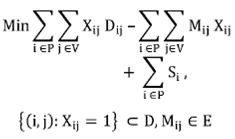
Objective Function (PII.1): the first term refers to the total Euclidean territory distance. The second term represents the alignment on preference allocation. The excess value of profit variance is the third term.
Unique-assignment-constraint: constraint (PII.2) assigns each BUj to one branch i only. This constraint is included in both Phases I and II because territory centers (i.e. branches) and BU's allocation may change in Phase II as well.
Activity-measure-side constraints: constraints (PII.3) are defined to ensure that each territory is within a maximal deviation from the capacity value
Traveling-distance constraint (PII.4): maximum distance δ i is allowed for end-customers assigned for branch i.
Branch-type constraint: constraint (PII.5) sets the minimum and maximum number of branches selected on incumbent solution for each type of branch b.
Alignment constraints: geographical issues like rivers or mountains are modeled explicitly as hard constraints in (PII.6). We explicitly enumerate into a subset F all pairs of BU's that cannot be assigned on the same territory.
Contiguity constraints: constraints (PII.7) guarantee connectivity of territories and were initially proposed in 20 to constrain connectivity in routing problems. It evaluates if a subset C contains a partition of BU's that are assigned to a territory center i but are disconnected from the rest of BU's assigned to the same territory. The cardinality of the subset C ranges from 1 up to H/2, where Η is the number of BU's assigned to the territory. The subset N c represents the union set of all BU's that are adjacent to any member of C. If BUj is assigned to territory i, at least one of the neighbors of BUj (i.e. q ∈ N c ) needs to be assigned to the same territory as BUj. In other words, at least one of the BU's q that is adjacent to any member of C must be assigned to the same territory i as it is with all the members of C. The main issue with connectivity is the exponential number of contiguity constraints, which makes it impossible to write them explicitly.
Profit variance excess constraint: constraint (PII.8) is defined to compute the excess profit variance when compared with the target profit variance for each branch.
2.5 Data Description
The MFI provided the data so the values D
ij
PV
j
and
Table 1 Data description
| Parameter | Number |
|---|---|
| Basic Units (y) | 10000 |
| Branches (p) | 500 |
| Activity Measure (m) | 3 |
| Type of branch (b) | 5 |
| Types of loan (/) | 3 |
Table 2 provides an understanding of the size of the problem. Our optimization model has more than 5,512,000 constraints (approx.) and 5,020,000 decision variables. In addition, the number of the contiguity constraints is exponential; thus, it is impossible to state these constraints explicitly. The computational time is prohibitively large for a practical business user application of this model. For instance, we could not find a feasible solution for our problem with the described data in as many as 48 hours. The large scale of the problem is our main justification for the need of heuristics.
Table 2 Parameters for the hybrid heuristic
| Hybrid heuristic parameters | Values |
|---|---|
| FACTOR = parameter for initial territory center design | 5,7 |
| KERNEL = the percentage of initial allocation assignments | 0 - 0.30 |
| PERT = objective function weight for perturbation | 500 - 10k |
| KVARS = variance weight factor among branches | 1k - 10k |
| CORE = proportion of branches that can be used for re-centering | 0.6 - 0.9 |
For a similar problem in a different context, 12 suggests a similar MIP program with 5,000 basic units and without considering the variability of the profit allocation, the computational time is prohibitively large and justified the need for heuristics. The following section introduces the solution framework and the proposed heuristics in detail.
3 Solution Framework: Hybrid Heuristic
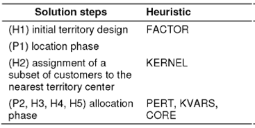
We utilize a solution procedure based on an iterative cut generation strategy within a branch and bound framework 21 to solve this large-scale mixed integer program. The computational time is prohibitively large for practical business application of this model. This manuscript presents a hybrid heuristic to solve large scale mixed integer programs. In addition to the heuristics that are proposed in 12, 19, we utilize novel heuristics for dynamic re-calculation of profit variability among territory centers and dynamic relocation of branches. Thus, heuristics (H1)-(H5) are utilized all together as a hybrid heuristic in order to reduce the search space and complexity (see Table 2 for the parameter definitions).
Prior to the location phase, a pre-processing heuristic for initial territory design using FACTOR parameter is utilized. After the solution of Problem 1, there is another pre-processing heuristic using the parameter KERNEL. Then, the rest of the heuristics, perturbation, and dynamic recalculation of profit variance among territory centers and dynamic relocation of branches are utilized to solve Problem 2. Table 3 lists the steps of the proposed solution framework.
Overall, initial territory center design is crucial since it can decrease the number of iterations to reach to an optimal solution. That is the main reason of utilizing Heuristic 1 and solving Problem 1. The second phase allocates the customers with respect to the activity measures while allowing dynamic updating of the territory centers. A cut-generation strategy is used to recursively evaluate the contiguity required by each territory. Consequently, the capacity and side constraints are updated depending on the branch type selected for territory centers. The following sub-sections discuss the proposed heuristics and their characteristics in detail.
3.1 H1: Pre-Processing Heuristic for Initial Territory Centers (FACTOR)
This pre-processing heuristic (H1) is used to simplify the network and design initial territory centers before solving Problem 1. The basic idea of the pre-processing heuristic for initial territory centers is to choose a subset of the connected branches for each customer group. Mathematically, the following criteria are used:

R is a subset of relevant arcs from D that are constructed using this pre-processing heuristic to reduce complexity. FACTOR serves as a capacity value of the respective activity measure for a particular branch. FACTOR is commonly set to 5 during our implementation.
3.2 H2: Pre-Processing Heuristic for Initial Allocation Assignments (KERNEL)
Heuristic H2 is utilized after the location phase and before solving Problem 2. The solution of Problem 1 provides the set of initial territory centers.
Then, heuristic H2 assigns a partition of geographic basic units to the nearest territory center belonging to the set of initial territory centers. This heuristic, which is based on setting a percentage of decision variables to one, can be formally presented as follows:
Let X ij, = 1 where {(i j)} ⊂ R ⊂ D such that

The use of heuristics for initial territory centers and for initial allocation assignments may result in a loss of optimality 19. That motivates us to utilize a heuristic that allows dynamic re-centering of the territories, which is presented as heuristic H5.
3.3 H3: Perturbation (PERT)
The perturbation heuristic has been shown to be effective for mixed integer programs, for instance, within the context of fleet assignment problems 21. The basic idea of this heuristic is to provide feedback to the objective function about customers already connected to a particular branch for which no changes are expected. This prevents assignment changes unless the improvement in the objective function is large.
Let the dynamic parameter Z
t
represent the number of basic units that are disconnected at each iteration t. In fact, it is expected that the parameter Z
t
would get smaller in the following iterations as a result of satisfying the added contiguity constraints (PII.7) Let U ⊂ R represent the subset of basic units (BUs) that are already connected to the territory center i. Therefore, the parameter
ObjFunc (t)
 PII.Ib
Where {(i,j): Xij = 1} ⊂ R ⊂ D,
MijE, U ⊂ R,
Z t = number of BU's that are disconnected at each iteration t.
The modified objective function (Pll.lb) is now defined at every iteration (ObjFunc (t) ). As a measure of compactness, the penalty term within the objective function for BUj is inversely proportional to D ij . That is, the smaller the distance of the jth BU to the ih territory center is, the larger the penalty term within the objective function becomes. This change avoids any assignment changes for the decision variable X ij . Smaller values of Ζ should lead to faster convergence to the optimal solution. Larger values of the perturbation parameter enforce the MIP objective function to keep the assignment of as it is by assigning a larger penalty. Perturbing costs can adversely affect the number of interior-point iterations required. In some cases, this increase in the number of interior iterations is expected to be offset by finding an optimal basis quickly. A value of zero for the perturbation parameter implies that the effect of the perturbation heuristic is negligible which may result in slower convergence. These three heuristics have been implemented for mixed integer programs in different contexts 12, 19.
3.4 H4: Dynamic Updating of Profit Variability Among Territory Centers (KVARS)
The variance weight factor KVARS is implemented within the objective function (PII.1) in order to assign a weight on the profit variability among branches. This heuristic modifies the objective function by replacing Σi∈ΡSi with Σi∈Ρ
We can implement a static or dynamic weight for variance through all iterations on the algorithm. This manuscript employs a static variance weight factor for which small (i.e. 500) values lead to larger weights for variance within the objective function and to lower profit variability among branches. However, a small static variance weight factor may produce a trade-off with the perturbation parameter and may result in slower or no convergence. Another strategy is to set a dynamic linear negative function for the variance weight factor that starts with an initial large value on the variance weight factor and decreases the value dynamically. Three parameters need to be determined for this dynamic strategy: (1) an initial variance weight factor value (kivars=5000), (2) a final value (kfvars=1000), and (3) a number of iterations to get the final value (kuvars=10). Our preliminary experiments provide evidence showing that this dynamic strategy can be very valuable while facing hard-tightened problems.
3.5 H5: Dynamic Relocation of Branches CORE
An optimal branch is by definition the block that has the smallest total distance to the set of customers assigned to the territory. Some constraints in Problems 1 and 2 are relaxed to determine the initial territory centers. This may lead to suboptimal territory centers. Thus, a dynamic relocation of branches is performed to ensure that the algorithm results with the optimal location for branches. This parameter (CORE) is used in order to define the subset of potential branches that can be used as candidates for territory re-centering.
In this heuristic Yi is recalculated in each iteration. When a branch i is re-located for any territory, then customers j distanced matrix is re-calculated accordingly for all relevant decision variables.
Consequently, constraints (PII.2), (PII.3), and (PII.4) should be redefined when a new branch is set as the territory center in any iteration. A large proportion of the branches are used for re-centering results in a larger local search for optimal branches as territory centers. Furthermore, it can be verified that fast convergence to the optimal solution is compromised as branch location is re-centered on territories. In fact, during the first iterations of the algorithm there is a lot of computational effort to find the optimal branch locations. After some iterations, re-location of centers is stabilized and then more effort and progress are reported on minimizing the profit variance among braches and minimizing compactness for territories. Similarly, for contiguity constraints, little progress is obtained on cut strategy contiguity constraints during branch relocation stage. This trade-off on dynamic relocation for territory centers prompts us not to start the re-location procedure during the first iterations. Therefore, we define a parameter inireloc that indicates the iteration number at which the algorithm starts applying the re-location strategy for the territory centers.
4 Performance of the Hybrid Heuristic and Further Desian of Experiments
This section evaluates the implementation of the hybrid heuristic to solve the utilized mixed integer program. The computer used for this implementation was a Dell IntelTM Core i7-3520; CPU 4 @ 2.90 Ghz; RAM 8GB; Windows-7 64 bits.
The hybrid heuristic was implemented on X- PRESS© MIP Solver from FICOTM (Fair Isaac, formerly Dash Optimization).
Firstly, we present evidence for the effectiveness of the hybrid heuristic. This is followed by an explanation of the design and purpose of the further experiments.
4.1 Performance of the Hybrid Heuristic
The large size and the complex constraint nature of the problem prevent us from having a feasible solution without any of the heuristics in as many as 48 hours. Therefore, the optimal solution is estimated by using a run with the minimal use of heuristics. For a FACTOR value of 5 and a perturbation heuristic parameter value of 12, a feasible solution for total Euclidean distance is retrieved within reasonable computational time.
This solution, 34.1029, is also the best solution that has been found as a result of extensive simulations. Therefore, we use it to estimate the optimal solution, and the percentage optimality gaps are computed using combinations of heuristic parameters.
Table 4 presents the optimality gaps for the cases where the FACTOR value is 5 and the variance weight factor is 10000. The reported optimality gaps are in the range of 0.47% and 3.17%, which is reasonable compared with the initial case where finding a feasible solution is difficult.
Table 4 Optimality gaps for runs with different combinations of parameter values
| KERNEL | CORE | PERT | Optimality Gap % |
|---|---|---|---|
| 0.00 | 0.00 | 1 | 0.5224% |
| 0.00 | 0.00 | 1 | 0.5897% |
| 0.00 | 0.00 | 1 | 0.4745% |
| 0.00 | 0.00 | 1 | 0.4562% |
| 0.00 | 0.00 | 17 | 0.9247% |
| 0.00 | 0.00 | 17 | 0.5224% |
| 0.00 | 0.00 | 17 | 0.5897% |
| 0.00 | 0.00 | 17 | 0.4745% |
| 0.00 | 0.00 | 17 | 0.4562% |
| 0.10 | 0.60 | 30 | 1.0417% |
| 0.20 | 0.60 | 30 | 0.6624% |
| 0.30 | 0.60 | 30 | 0.5799% |
| 0.10 | 0.90 | 30 | 0.9610% |
| 0.20 | 0.90 | 30 | 0.8712% |
| 0.30 | 0.90 | 30 | 0.4748% |
| 0.00 | 0.90 | 50 | 1.2958% |
| 0.10 | 0.90 | 50 | 1.8331% |
| 0.20 | 0.90 | 50 | 1.3563% |
| 0.30 | 0.90 | 50 | 1.0480% |
| 0.00 | 0.90 | 100 | 2.2358% |
| 0.10 | 0.90 | 100 | 2.2674% |
| 0.20 | 0.90 | 100 | 3.1534% |
| 0.30 | 0.90 | 100 | 2.9326% |
| 0.00 | 0.90 | 110 | 2.3304% |
| 0.30 | 0.90 | 110 | 2.7110% |
| 0.00 | 0.90 | 130 | 3.1693% |
| 0.00 | 0.99 | 1 | 0.3183% |
| 0.00 | 0.99 | 1 | 0.0507% |
| 0.00 | 1.50 | 1 | 0.0079% |
| 0.00 | 0.99 | 1 | 0.4690% |
| 0.00 | 1.25 | 1 | 0.1095% |
| 0.00 | 0.99 | 1 | 0.2731% |
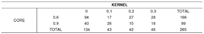
Table 7 Levels for experimental design factors PERT and KVARS
| Parameter | Minimum | Median | Maximum |
| PERT | 30 | 90 | 150 |
| KVARS | 500 | 5000 | 10000 |
The next subsection describes the design of the experiment that aims to provide sensitivity analysis.
4.2 Design of Experiments
Our preliminary experience has shown that the proposed large scale mixed integer program is challenging to solve. We proposed a hybrid heuristic and now investigate the sensitivity of the solution to the heuristic parameters. The main purpose of the further experiments is to understand how to choose the hybrid heuristic parameters KERNEL, PERT, KVARS, and CORE. Particularly, the objective is to analyze the trade-offs between the quality of the solution and the computational time with respect to the choice of these parameters. The quality of the solution is measured by
the total Euclidean distance (MIPSOL), also referred to as compactness, and
the resulting profitability variance among branches (VARS).
The solutions with a smaller total Euclidean distance and a smaller profitability variance among branches are deemed to be of high quality. We aim to provide some insights about the choice of the heuristic parameter values that increase the efficiency of the search.
5 Analysis
This section provides graphical and statistical analyses based on the described experimental design. The objective is to evaluate the patterns of the relationship among the four hybrid heuristic parameters KERNEL, PERT, KVARS, and CORE and three performance indicators: (1) the compactness of the solution, (2) the resulting profitability variance among branches, (3) the length of the computational time.
Locally weighted regression (loess) analysis was used via the R software package 23. Loess is a non-parametric regression method for fitting a regression surface to data through multivariate smoothing 24. After presenting the computational results, a discussion is provided in order to share the gained insights.
5.1 Computational Results
Figure 2 shows the influence of the perturbation parameter on compactness of the solution while controlling the size of the area searched for optimal territory centers (CORE). It should be noted that, for illustration purposes, the variance weight factor was discretized as terciles with respect to its empirical distribution (i.e., [500, 5000) [5000, 6000) [6000, 10000]). In general, an increase in the perturbation parameter results in less compact solutions.
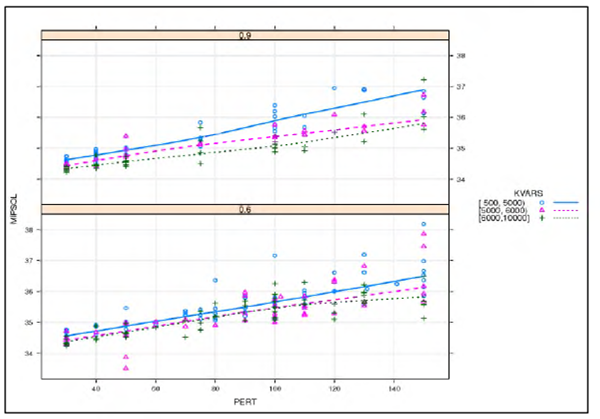
The effect of the variance weight factor on the compactness is directly proportional to the size of the area searched for optimal territory centers. Therefore, a significant part of the variability in the solution compactness is explained by the magnitude of the perturbation factor, and to a lesser extent by the magnitude of the variance weight factor KVARS.
Larger variance weight factor values result in more compact solutions as shown in Figure 2. An increase in the area searched for optimal territory centers in conjunction with an increase in the variance weight factor also leads to more compact solutions.
Figure 3 shows how the compactness of the solution varies across the range of values for the parameter of initial allocation assignment (KERNEL) that fixes a subset of Xij-binary variables as one. It is shown that smaller values for the magnitude of the variance weight factor results in solutions with larger total Euclidean distances.
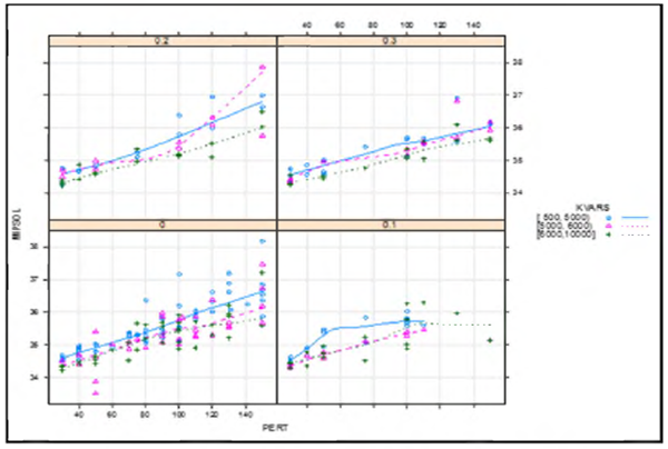
For a larger number of initial allocation assignments during the pre-processing phase, the larger magnitudes of the variance weight factor (observe the dotted line) are more consistently associated with more compact solutions.
There is more variability in the compactness of the solution for a larger number of initial allocation assignments (0.30). The variability of the compactness of the solution also increases with larger perturbations. Regardless of the magnitude of the variance weight factor, for a larger percentage of initial allocation assignments during pre-processing (0.30), the variability of the compactness of the solution is smaller.

We fit linear models to evaluate the magnitude of the relationships observed in the graphical analysis. Interaction effects between parameters are also considered in the models for non-linear patterns. Non-parametric bootstrap interval estimators 25 were generated for each slope coefficient, as a remedy to the violations of the Gauss-Markov Theorem in the residuals.
Graphical analyses to evaluate the effect of the hybrid heuristic parameters on the profitability variance among branches (VARS) are shown in Figures 5 and 6. Determining the percentage of initial allocation assignments during preprocessing as 0 results in a positive linear pattern for the profitability variance among branches and perturbation. Setting the percentage of the initial allocation assignments during pre-processing to 0.2 and 0.3 leads to curvilinear relationships between the heterogeneity of the profitability, profitability variance among branches, and perturbation (see Figure 5). There is also evidence implying that an increase in the variance weight factor is associated with an increase in profitability variance among branches (see Figure 6). Indeed, most of the variation in the resulting profitability variability can be explained by the magnitude of the variance weight factor.
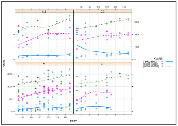

Table 9 shows the non-parametric bootstrap slope estimates resulting from 1000 replications for a linear model, including second order interaction effects, to estimate profitability variance among branches as a function of 1) the size of the area searched for optimal territory centers, 2) the percentage of initial allocation assignments, 3) perturbation, and 4) variance weight factor. These bootstrap estimates support some of the patterns observed in Figures 5 and 6 such as the positive relationship between profitability variance among branches and perturbation, the positive relationship between the variance weight factor, and the difference in patterns for profitability variance among branches for the various percentages of initial allocation assignments. The regression model suggests with a 95% confidence that the proportion of the variability in profitability variance among branches explained by these parameters is contained in the interval (88%, 93%). Figure 7 shows the proportion of R2 loss if the variable is removed. The resulting profitability variability is explained by the magnitude of the variance weight factor.

Table 8 Bootstrap estimates for the slope coefficients: MIPSOL
| Coefficients | 95% Int.estimates |
|---|---|
| Intercept | (33.90, 34.29 ) |
| CORE = 0.9 | ( 0.0134, 0.2908 ) |
| KERNEL = 0.1 | (-0.1884, 0.5843 ) |
| KERNEL = 0.2 | (-0.2764, 0.3426 ) |
| KERNEL = 0.3 | (-0.1336, 0.3427 ) |
| PERT | ( 0.0153, 0.0197 ) |
| KVARS | (-0.0001, 0.0000 ) |
| CORE=0.9*KVARS | (-0.0001, 0.0000 ) |
| KERNEL=0.1*PERT | (-0.0087, 0.0000 ) |
| KERNEL=0.2*PERT | (-0.0040, 0.0048 ) |
| KERNEL=0.3*PERT | (-0.0066, -0.0006 ) |
| KERNEL=0.1*KVARS | ( 0.0000, 0.0001 ) |
| KERNEL=0.2*KVARS | (0, 0) |
| KERNEL=0.3*KVARS | (0, 0) |
| df=251 | R2 =(0.6789, 0.784) |
Table 9 Bootstrap estimates for slope coefficients: VARS
| Coefficients | 95% Int.estimates |
|---|---|
| Intercept | (-548.2, -242.5 ) |
| CORE = 0.9 | (-391.1, 14.8) |
| KERNEL=0.1 | ( 14.4, 607.8 ) |
| KERNEL=0.2 | (162.9, 892.9 ) |
| KERNEL=0.3 | (422.7, 1434.7 ) |
| PERT | ( 2.924, 6.117 ) |
| KVARS | ( 0.2704, 0.2980 ) |
| CORE=0.9*KERNEL=0.1 | (-307.5, 40.0 ) |
| CORE=0.9*KERNEL=0.2 | (-560.5, -46.8 ) |
| CORE=0.9*KERNEL=0.3 | (-740.1, -234.0 ) |
| CORE=0.9*PERT | ( 0.581, 5.376 ) |
| CORE=0.9*KVARS | (-0.0235, 0.0224 ) |
| KERNEL=0.1*PERT | (-4.084, 1.508 ) |
| KERNEL=0.2*PERT | (-4.796, 2.259 ) |
| KERNEL=0.3*PERT | (-7.490, -0.705 ) |
| KERNEL=0.1*KVARS | (-0.0404, 0.0087 ) |
| KERNEL=0.2*KVARS | (-0.0532, 0.0112 ) |
| KERNEL=0.3*KVARS | (-0.0669, 0.0121 ) |
| df = 247 | R2 = ( 0.8790, 0.9279 ) |
Table 10 shows non-parametric bootstrap slope estimates resulting from 1000 replications for the model (including second order interaction effects) to estimate computational time as a function of 1) the size of the area searched for optimal territory centers, 2) the percentage of initial allocation assignments, 3) perturbation, and 4) variance weight factor.
Table 10 Bootstrap estimates for slope coefficients: TIME
| Coefficients | 95% Int.estimates |
|---|---|
| Intercept | ( 5078, 15823 ) |
| CORE = 0.9 | (-2395.7, 1520.5 ) |
| KERNEL=0.1 | ( 1034, 14340 ) |
| KERNEL=0.2 | (203,6832 ) |
| KERNEL=0.3 | (925, 8442 ) |
| PERT | (-471.9, -55.1 ) |
| PERT2 | (0.553, 5.488 ) |
| PERT3 | (-0.0180, 0.0003 ) |
| KVARS | (-0.5607, 0.0286 ) |
| PERT*KVARS | (-0.0011, 0.0054 ) |
| CORE=0.9*KERNEL=0.1 | (-3876.7, 2833.4 ) |
| CORE=0.9*KERNEL=0.2 | (-3055.9, 1381.6 ) |
| CORE=0.9*KERNEL=0.3 | (-118, 4968 ) |
| CORE=0.9*PERT | (-13.2, 39.2) |
| KERNEL=0.1*PERT | (-96.66, 8.17 ) |
| KERNEL=0.2*PERT | (-28.385, 40.413 ) |
| KERNEL=0.3*PERT | (-69.68, -7.37 ) |
| KERNEL=0.1*KVARS | (-0.7587, 0.0249 ) |
| KERNEL=0.2*KVARS | (-0.5378, 0.0212 ) |
| KERNEL=0.3*KVARS | (-0.6398, -0.0518 ) |
| df = 245 | R2 (0.2208, 0.3525) |
A graphical analysis for the hybrid heuristic parameters appears in Figure 8. Larger values of the perturbation factor are associated with larger computational time. However, larger values of the variance weight factor are associated with faster convergence. This pattern is more pronounced for a larger area searched for optimal territory centers (CORE=0.90).
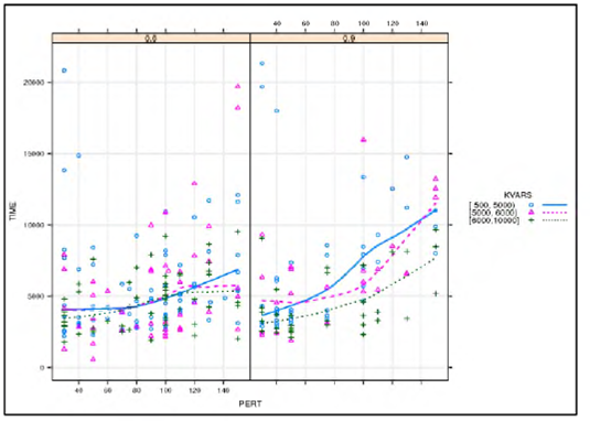
The relationships among the parameters and completion time are non-linear, see Figure 8. For large percentages of initial allocation assignments during pre-processing, the better computational times are also associated with the larger values of the variance weight factor. Figure 9 provides evidence that larger values of the size of the area searched for optimal territory centers, percentage of initial allocation assignments during preprocessing, and the magnitude of the variance weight factor are associated with a solution of better compactness and faster convergence.

These bootstrap estimates support patterns observed in Figures 8 and 9 such as the curvilinear relationship between computational time and perturbation, and the changes in the relationships between the magnitude of the variance weight factor, perturbation, and time for different values of percentage of initial allocation assignments,
The regression model suggests with a 95% confidence that the proportion of the variability in computational time explained by these parameters is contained in the interval (22%, 35%). Figure 10 shows the proportion of R2 loss if the variable is removed. Omitting the percentage of initial allocation assignments during pre-processing or perturbation from the model results in the loss of about half of the explanatory power of computational time. Likewise, omitting the magnitude of the variance weight factor will drop the explanatory power of the model more than by 35%.

5.2 Discussion of the Results
The experiment shows that, in general, there is a complex interaction between these heuristics and the overall performance. Our evidence shows that the heuristics can be fine-tuned to improve the quality of the optimal solution as well as the length of the computational time.
Concerning the effect on compactness, in general, lower perturbation parameters and larger variance weight factors lead to more compactness. The negative effect of increasing perturbation on compactness is moderated (stabilized) by compactness is also improved by increasing the adjusting the percentage of initial allocation search area for optimal territory centers, assignments during pre-processing. The compactness is also improved by increasing the search area for optimal territory centers.
With regards to the effect on profitability of profitability is greatly influenced by the variance among branches, naturally, the variance weight factor. An increase in perturbation decreases the variance of profitability for a larger percentage of initial allocation assignments during pre-processing. The profitability variance also decreases if the percentage of initial allocation assignments during pre-processing and the search area for optimal territory centers are relatively large.
Concerning the effects on computational time, in general, larger values of the variance weight factor are associated with faster convergence.
The speed of convergence is heavily influenced by the pre-processing heuristic.
5.3 Managerial Insights
In addition to the computational test for heuristics, a method to understand a representation of the solution is determined as a requirement for business users before implementation. We used a GIS application in order to make a graphical representation of our territory design solution. This strategy was useful not only to demonstrate how the business rules are considered on the proposed solution, particularly, for risk balance constraints, but also to figure out any other potential operational difficulties during implementation. Figure 11 includes an example of a real-world solution implemented for the MFI. Because of size and complexity issues, we show a partial map of the entire territory design for presentation.
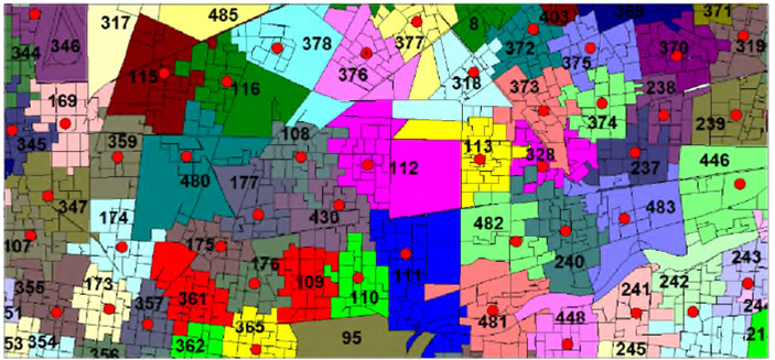
Each territory has a number-ID and a branch location indicated with a red point. From this drawing we can easily determine the compactness of the territories. Since we have activity measure constraints and risk balance constraints, it is clear that contiguity and compactness are compromised. The balance of basic units among territories can be visually recognized although it is not required.
The proposed model provides near optimal solutions to the problem. This is true not only because our approach considers all the real world constraints from business requirements, but in addition we take particular focus on risk balancing for territory design. Furthermore, on each iteration during the branch and cut framework, we obtain solutions that are lower bound solutions to the relaxed problem without contiguity constraints. This strategy assures a near optimal solution. Finally, the dynamic re-location approach for territory center location offers the business a selection for territory branches not only from geographic perspective but in terms of capacities and balance as well. The additional managerial implications include potential changes of compactness due to changes of demand from new customers and lower capacity because of the closure of branches. This may need to be addressed in a dynamic manner along with the development of the market. The existing model can be updated accordingly with respect to the practical needs of the MFI.
6 Conclusions and Future Work
Micro finance has emerged in the early 21st century as a solution to scarce capital in countries with developing economies. One of the key elements in micro financing is accessibility to the funds. The allocation of branches for these micro finance institutions presents a difficult task.
This manuscript addresses an actual territory design problem faced by a large-size micro financial firm. In this territory allocation problem, two main decisions have been identified: location of branches for territory centers and allocation of end customers to each territory center. For a robust territory design, profit variability, measure of risk among branches is minimized. This real world problem was modeled using a large scale mixed integer program which is solved with a hybrid heuristic approach. These heuristics were implemented within a recursive branch and cut procedure to solve this ΝP-hard complete problem. The high computational cost for an exact optimal solution justifies the heuristic approach.
The value of the hybrid heuristic approach to solve large scale mixed integer programs with hard/complex constraints is shown by the computational results.
We provide a comprehensive statistical analysis regarding the choice of the parameters. The impact of the hybrid heuristic parameters is analyzed using (1) territory design compactness, (2) variance of the profitability among branches, and (3) total computational time. The proportion of branches that can be used for re-centering, the perturbation parameter, and the variance weight factor are found to have a significant impact on territory design compactness. It has been observed that the perturbation parameter accounts for most of the variability in compactness. Therefore, one needs to be careful about choosing the perturbation parameter if the quality of the solution is the main concern rather than the computational time.
Moreover, the percentage of initial allocation assignments, perturbation and variance weight parameters are found to have a significant impact on the profitability variance. The variance weight factor, relative weight on the penalized objective function for heterogeneity among branches, accounts for most of the variability in profitability variance. The negative impact of initial allocation assignments on profit variability among branches implies that larger search spaces and more complexity show increased profit variance among branches.
Lastly, we can suggest that the covariance model is not significantly able to capture the complexity of the relationship among the completion time and the parameters, which is observed in the graphical analysis. Nevertheless, the covariance model provides interesting insights. For instance, we found that larger values of the perturbation parameter are convexly associated with the computational time. Contrary to what was expected, positive associations between the perturbation parameter and computational time and between the percentage of initial allocation assignments and computational time have been detected. The increases in convergence time with increasing values of the perturbation parameter and the percentage of initial allocation assignments are moderated by the interaction of the percentage of initial allocation assignments and variance weight parameters. We have got graphical evidence suggesting that larger values of percentage of initial allocation assignments, the proportion of branches that can be used for re-centering, and the variance weight factor are associated with better quality solutions (compactness) and faster convergence. This especially occurs for larger values of the variance weight factor.
Our future research will include an exploration of the complex behavior of computational time and optimality for solution spaces with higher levels of profitability heterogeneity. We can also utilize a dynamic linear negative function for the variance weight factor that starts with an initial large value and seeks for smaller variance weight factor values at iterations without an improvement in the overall variance. Our initial computational experience provides positive evidence that this dynamic strategy can be valuable in terms of decreasing the computational time with lower profit variability. Future work will also include a simulator for the second phase. As of now, we have investigated the feasibility of the consideration of uncertainty within the model and explored potential ways to solve that model.
In conclusion, this manuscript presents a hybrid heuristic solution to a territory design problem in MFI literature by adding the consideration of both mean and variance of profit allocation to the existing mixed integer programming models. The experimental design and computational instances provide insights about the behavior of the heuristics within the proposed setting and show their effectiveness.

